How to Calculate Q1 and Q3: The Definitive Statistical Guide for Precision Analysis
Understanding how to calculate Q1 and Q3 is foundational for anyone working with statistical data. These quartiles divide datasets into four equal parts, revealing distribution patterns that simple averages miss. Without precise quartile calculations, insights into data spread—critical for fields like finance, healthcare, and market research—remain obscured. The stakes are higher than most realize: incorrect quartile values can distort risk assessments, skew performance metrics, and mislead decision-makers.
Many professionals rely on software to compute quartiles, but true mastery requires grasping the underlying mechanics. Whether you're analyzing stock volatility, patient response rates, or customer spending habits, knowing how to calculate Q1 and Q3 manually ensures accuracy when tools fail or when custom methods are needed. The difference between a method like the Tukey hinge and the Moore-Greenhouse approach isn’t just academic—it can alter conclusions entirely.
The confusion often stems from conflicting definitions. Some textbooks define quartiles as dividing data into four equal groups, while others treat them as percentiles (25th and 75th). This ambiguity leads to discrepancies in reports, especially when comparing datasets across industries. Below, we clarify the standard methods, historical context, and practical applications—so you can apply quartile calculations with confidence.

The Complete Overview of How to Calculate Q1 and Q3
Quartiles are statistical benchmarks that split ordered data into four segments, each containing 25% of observations. Q1 (the first quartile) marks the 25th percentile, while Q3 (the third quartile) represents the 75th percentile. Together, they define the interquartile range (IQR), a robust measure of data dispersion that resists outliers—a critical advantage over standard deviation in skewed distributions.The process of how to calculate Q1 and Q3 hinges on two key steps: ordering the dataset and applying a specific interpolation formula. Unlike the median (Q2), which is straightforward, quartiles require careful handling of even/odd datasets and edge cases. Missteps here can lead to inconsistent results, particularly when datasets have repeated values or gaps. For instance, a dataset with 100 values will yield Q1 at the 25th position, but a dataset with 101 values demands interpolation between the 25th and 26th values.
Historical Background and Evolution
The concept of quartiles emerged in the 19th century as statisticians sought to quantify data distribution beyond simple averages. Early methods, such as those proposed by Francis Galton, treated quartiles as exact percentiles, dividing data into four equal parts by position. However, this approach proved cumbersome for large datasets, prompting later mathematicians to refine interpolation techniques.By the mid-20th century, statisticians like Harold Hotelling and George W. Snedecor formalized quartile calculation methods, emphasizing linear interpolation for precise placement. Today, how to calculate Q1 and Q3 follows standardized formulas (e.g., the Method of Hyndman and Fan), though variations persist across software packages. For example, Excel’s `QUARTILE` function uses a different algorithm than R’s `quantile()`, leading to discrepancies in reported values—a detail that can have real-world consequences in fields like climate science or medical research.
Core Mechanisms: How It Works
The standard method for calculating quartiles involves:1. Sorting the dataset in ascending order.
2. Determining positions using the formula:
\[
P = \frac{(n-1) \times p}{100}
\]
where \( n \) is the dataset size and \( p \) is the percentile (25 for Q1, 75 for Q3).
3. Interpolating if \( P \) is not an integer, typically via linear interpolation between adjacent values.
Table of Contents
- The Complete Overview of How to Calculate Q1 and Q3
- Historical Background and Evolution
- Core Mechanisms: How It Works
- Key Benefits and Crucial Impact
- Major Advantages
- Comparative Analysis
- Future Trends and Innovations
- Conclusion
- Comprehensive FAQs
- Q: Why do different software tools (Excel, R, Python) give different Q1/Q3 values?
- Q: Can Q1 and Q3 be calculated for non-numeric data?
- Q: How does sample size affect quartile calculation?
- Q: What’s the difference between quartiles and percentiles?
- Q: When should I use quartiles instead of mean/standard deviation?
For example, in a dataset of 20 values:
This method ensures consistency, but alternatives (e.g., the nearest rank method) may yield slightly different results. Understanding these nuances is essential when how to calculate Q1 and Q3 must align with industry standards or regulatory requirements.
Key Benefits and Crucial Impact
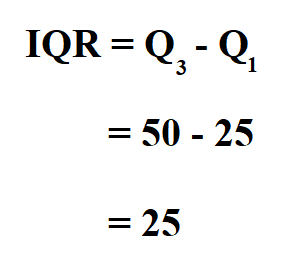
Quartiles are indispensable tools for summarizing data distributions, particularly in scenarios where outliers distort traditional measures like mean and standard deviation. They form the backbone of box plots, enabling visual comparisons of spread and skewness across datasets. In finance, Q1 and Q3 help identify market quartiles for portfolio diversification, while in healthcare, they assess patient response variability to treatments.The interquartile range (IQR = Q3 – Q1) is especially valuable for detecting anomalies. A dataset with an IQR of 10 but a standard deviation of 50 suggests heavy-tailed data—information critical for risk management. Without precise quartile calculations, such insights would remain hidden, leading to suboptimal strategies.
"Quartiles are the silent guardians of data integrity—they reveal what the mean conceals." — John Tukey, Statistician
Major Advantages
- Robustness to Outliers: Unlike mean/standard deviation, quartiles focus on central data trends, making them ideal for skewed distributions.
- Visual Clarity: Box plots use Q1, Q3, and median to display data spread intuitively, aiding exploratory analysis.
- Regulatory Compliance: Industries like finance and healthcare mandate quartile-based reporting for transparency.
- Software Flexibility: Mastering manual calculations ensures accuracy when tools (e.g., Excel, Python) use non-standard methods.
- Decision-Making Precision: Quartiles help set performance benchmarks (e.g., "top 25% of sales") without arbitrary cutoffs.

Comparative Analysis
| Method | Description |
|---|---|
| Linear Interpolation (Hyndman-Fan) | Standard for most statistical software; interpolates between adjacent values for non-integer positions. |
| Nearest Rank | Rounds to the nearest integer position; simpler but less precise for small datasets. |
| Tukey’s Hinge | Used in exploratory data analysis; median of lower/upper halves, ignoring middle value for odd \( n \). |
| Excel’s QUARTILE | Uses a proprietary algorithm (Method 1: linear; Method 2: nearest rank), differing from R/Python. |
Future Trends and Innovations
As big data grows, quartile calculations are evolving to handle high-dimensional datasets. Machine learning models now use quantile regression to predict Q1/Q3 directly, bypassing traditional interpolation. Additionally, dynamic quartile methods (e.g., adaptive binning) adjust to streaming data, critical for real-time analytics in IoT and finance.The rise of quantile forests—ensemble methods for robust quartile estimation—promises to reduce sensitivity to outliers further. Meanwhile, regulatory bodies are standardizing quartile definitions to minimize cross-platform inconsistencies, ensuring how to calculate Q1 and Q3 remains a universal benchmark.
Conclusion
Quartiles are more than statistical curiosities—they are the bedrock of data-driven decision-making. Whether you’re analyzing market trends, clinical trials, or operational efficiency, knowing how to calculate Q1 and Q3 with precision is non-negotiable. The choice of method depends on context: linear interpolation for general use, Tukey’s hinges for exploratory analysis, or software-specific adjustments for compliance.As data complexity increases, so too must the rigor of quartile calculations. The tools and techniques outlined here equip you to navigate this landscape confidently—ensuring your insights are both accurate and actionable.
Comprehensive FAQs
Q: Why do different software tools (Excel, R, Python) give different Q1/Q3 values?
A: Each tool uses a distinct quartile calculation method. Excel’s `QUARTILE` defaults to Method 1 (linear interpolation), while R’s `quantile()` uses Type 7 (nearest rank). Python’s `numpy.percentile` follows Hyndman-Fan by default. Always specify the method to ensure consistency.
Q: Can Q1 and Q3 be calculated for non-numeric data?
A: No. Quartiles require ordered, numeric data. Categorical or ordinal data (e.g., survey responses) must be encoded numerically first or analyzed using alternative methods like median splits.
Q: How does sample size affect quartile calculation?
A: Smaller datasets (<30 values) are more sensitive to interpolation methods. For \( n = 10 \), Q1 might be the 3rd value (nearest rank) or interpolated between the 2nd and 3rd (linear). Larger datasets converge to similar results across methods.
Q: What’s the difference between quartiles and percentiles?
A: Quartiles are specific percentiles (Q1 = 25th, Q2 = 50th, Q3 = 75th). Percentiles generalize to any value (e.g., 90th percentile). Quartiles are used for division into four parts; percentiles for finer granularity.
Q: When should I use quartiles instead of mean/standard deviation?
A: Use quartiles when data is skewed, contains outliers, or you need a robust measure of central tendency. Mean/standard deviation are appropriate for symmetric, normally distributed data without extreme values.
Leave a Comment
Comments are moderated before appearing. The data you submit is processed according to the Privacy Policy of Gouv.