What Is Correlation Coefficient? The Hidden Math Behind Relationships in Data
The numbers don’t lie, but they rarely speak plainly. Behind every scatterplot’s upward drift lies a silent arbiter: the correlation coefficient. This single value—often overlooked in favor of flashier visuals—quantifies the strength and direction of relationships between variables, from stock market trends to human behavior. It’s the bridge between raw data and actionable insight, yet its nuances remain misunderstood even among professionals who wield it daily.
Consider this: a pharmaceutical company discovers that patients with higher blood pressure respond better to a new drug. The correlation coefficient doesn’t just say "they’re linked"—it specifies how tightly and in what direction. Is the relationship linear? Exponential? Weak enough to dismiss? The answer lies in this statistical workhorse, a tool as precise as it is deceptively simple. Misinterpret it, and you risk drawing conclusions from noise; master it, and you unlock a lens to see patterns others miss.
The correlation coefficient isn’t just a relic of academic textbooks. It’s the quiet force behind algorithmic trading, climate science projections, and even social media engagement models. Yet for all its ubiquity, its true power lies in its limitations—and understanding those boundaries is where true expertise begins.

The Complete Overview of What Is Correlation Coefficient
The correlation coefficient is a standardized measure of the linear relationship between two continuous variables, ranging from -1 to 1. When two datasets move in lockstep—like ice cream sales and sun exposure—you’ll find a coefficient near +1. Conversely, a -1 suggests an inverse dance: as one variable rises, the other falls predictably. At 0, the variables are statistically independent, though not necessarily causally unrelated. This numerical compass doesn’t just describe relationships; it quantifies their reliability, offering a framework to distinguish between meaningful trends and random fluctuations.What sets the correlation coefficient apart is its dual role as both a descriptive statistic and a diagnostic tool. It doesn’t explain why variables correlate—only how strongly they do. This distinction is critical: a high correlation between ice cream sales and drowning incidents doesn’t imply causation (though it might suggest a third variable, like summer heat). The coefficient’s true value lies in its ability to filter signal from noise, providing a numerical anchor for decisions that would otherwise rely on subjective interpretation.
Historical Background and Evolution
The concept of measuring relationships between variables emerged in the late 19th century, but its modern form owes much to Karl Pearson’s 1896 work on the product-moment correlation coefficient—now universally called the Pearson correlation coefficient. Pearson’s innovation was to standardize the covariance between two variables by their respective standard deviations, creating a dimensionless metric that could be compared across datasets. Before this, researchers relied on vague descriptors like "strong" or "weak" relationships, leaving interpretation to individual bias.The Pearson coefficient’s dominance persisted until the mid-20th century, when statisticians like Maurice Kendall and Charles Spearman introduced alternatives for non-linear relationships. Spearman’s rank correlation, for instance, measures monotonic associations—useful when data violates the linearity assumption. These developments weren’t just academic refinements; they reflected a growing need for robustness in fields like psychology and economics, where real-world data rarely conforms to idealized models. Today, the correlation coefficient exists in a family of tools, each tailored to specific data characteristics, yet all rooted in Pearson’s original insight: that numbers, when properly aligned, can reveal invisible threads connecting disparate phenomena.
Core Mechanisms: How It Works
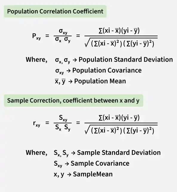
At its core, the correlation coefficient calculates the covariance between two variables and normalizes it by their standard deviations. Covariance measures how much two variables change together, but its absolute value depends on the units of measurement—making direct comparisons impossible. Dividing by standard deviations resolves this, yielding a unitless ratio. For Pearson’s r, the formula is:Table of Contents
- The Complete Overview of What Is Correlation Coefficient
- Historical Background and Evolution
- Core Mechanisms: How It Works
- Key Benefits and Crucial Impact
- Major Advantages
- Comparative Analysis
- Future Trends and Innovations
- Conclusion
- Comprehensive FAQs
- Q: What is correlation coefficient, and how is it different from covariance?
- Q: Can a correlation coefficient of 0 mean no relationship?
- Q: Why does sample size affect correlation significance?
- Q: How do I interpret a correlation coefficient of -0.7?
- Q: What are common mistakes when using what is correlation coefficient?
\[ r = \frac{\sum{(X_i - \bar{X})(Y_i - \bar{Y})}}{\sqrt{\sum{(X_i - \bar{X})^2} \sum{(Y_i - \bar{Y})^2}}} \]
Here, \(X_i\) and \(Y_i\) are individual data points, and \(\bar{X}\), \(\bar{Y}\) are their means. The numerator captures shared variance, while the denominator ensures the result is bounded between -1 and 1. Spearman’s rank correlation replaces raw values with their ranks, preserving the monotonic relationship’s integrity even when linearity fails.
The coefficient’s symmetry is a double-edged sword: swapping variables doesn’t change r, but this property can obscure directional nuances. For example, if X causes Y, the correlation is identical to Y causing X—a critical caveat when inferring causality. Moreover, outliers can distort r disproportionately, as a single extreme value can inflate or deflate the covariance without affecting standard deviations proportionally. This sensitivity underscores why visual inspection (e.g., scatterplots) remains essential alongside numerical results.
Key Benefits and Crucial Impact
The correlation coefficient’s utility spans disciplines, from medicine to machine learning, because it transforms abstract relationships into quantifiable insights. In healthcare, it might reveal that blood sugar levels and insulin resistance correlate at r = 0.87, guiding treatment protocols. In finance, a portfolio manager might use it to diversify assets by selecting securities with low r values, reducing risk. Even in social sciences, psychologists rely on it to validate survey responses—does self-reported happiness (X) align with measurable cortisol levels (Y)?Its impact extends beyond analysis into decision-making. A correlation coefficient of r = 0.6 between customer spending and ad exposure doesn’t just describe a trend; it justifies budget allocations. Similarly, climate scientists use it to correlate CO₂ levels with global temperatures, lending weight to policy arguments. The coefficient’s precision turns qualitative observations into actionable metrics, bridging the gap between theory and practice.
"Correlation is not causation, but causation is a subset of correlation." — Nassim Nicholas TalebThis aphorism encapsulates the coefficient’s paradox: it’s both a tool and a warning. While it cannot prove cause-and-effect, it identifies relationships worthy of deeper investigation. The danger lies in treating r as a standalone verdict—ignoring confounding variables, sample size, or temporal precedence. Yet when wielded with context, the correlation coefficient becomes a compass, pointing toward questions that define entire fields of study.
Major Advantages
- Standardization: The unitless scale (-1 to 1) allows comparisons across datasets with different units (e.g., correlating temperature in Celsius with ice cream sales in dollars).
- Directionality: The sign (+/-) immediately indicates whether variables move in tandem or opposition, aiding rapid interpretation.
- Statistical Rigor: Paired with hypothesis testing (e.g., t-tests), it quantifies whether observed correlations are statistically significant or due to chance.
- Non-Parametric Options: Spearman’s ρ and Kendall’s τ extend its use to ordinal data or non-linear relationships, broadening applicability.
- Foundation for Modeling: Many predictive algorithms (e.g., linear regression) rely on correlation coefficients to identify key input variables.
Comparative Analysis
| Pearson Correlation (r) | Spearman Rank (ρ) |
|---|---|
| Measures linear relationships between continuous variables. | Assesses monotonic relationships (linear or non-linear) via ranked data. |
| Sensitive to outliers; assumes normality. | Robust to outliers; works with non-normal distributions. |
| Optimal for normally distributed data. | Preferred for ordinal data or small samples. |
| Range: -1 to 1. | Range: -1 to 1 (interpretation similar to r). |
Future Trends and Innovations
As data grows more complex, the correlation coefficient’s role is evolving. Traditional r values are being supplemented by measures like partial correlation, which isolates relationships while controlling for third variables—a critical advancement in fields like genomics. Meanwhile, machine learning’s rise has spurred interest in non-linear correlation metrics, such as mutual information, which capture dependencies beyond linear trends.The future may also see greater integration with causal inference frameworks, where correlation coefficients serve as stepping stones to probabilistic causal graphs. Tools like Granger causality (for time-series data) or structural causal models could redefine how we interpret r, shifting focus from "are they related?" to "how do they influence each other?" Yet, for all these innovations, the core principle remains: the correlation coefficient is a lens, not a microscope. Its power lies in what it reveals—and what it leaves unsaid.

Conclusion
The correlation coefficient is more than a statistical curiosity; it’s a language for describing the unseen connections that shape our world. From Pearson’s original formulation to today’s algorithmic refinements, its journey mirrors humanity’s quest to impose order on chaos. Yet its true value lies not in the number itself, but in the questions it provokes: Why do these variables move together? What hidden mechanisms drive this relationship?Misused, it can mislead; mastered, it illuminates. The key is context—pairing numerical results with domain knowledge, visualizations, and causal reasoning. In an era drowning in data, the correlation coefficient remains a beacon, guiding researchers from correlation to causation, one step at a time.
Comprehensive FAQs
Q: What is correlation coefficient, and how is it different from covariance?
The correlation coefficient (r) standardizes covariance by dividing it by the product of the variables’ standard deviations, yielding a unitless measure between -1 and 1. Covariance, by contrast, retains the original units and lacks interpretability across datasets. For example, covariance between height (cm) and weight (kg) is meaningless without normalization.
Q: Can a correlation coefficient of 0 mean no relationship?
Not necessarily. A coefficient of 0 indicates linear independence, but variables may still relate non-linearly (e.g., Y = X²). Always visualize data (e.g., scatterplots) to check for hidden patterns.
Q: Why does sample size affect correlation significance?
Even weak correlations (e.g., r = 0.1) can achieve statistical significance in large samples due to reduced variance in the sampling distribution. Significance tests (e.g., t-tests) account for sample size, but practical significance—whether r matters in real-world terms—requires domain judgment.
Q: How do I interpret a correlation coefficient of -0.7?
A value of -0.7 indicates a strong inverse linear relationship: as one variable increases, the other decreases predictably. The magnitude (0.7) suggests a high degree of shared variance (~49%, via r²), but causation remains unproven.
Q: What are common mistakes when using what is correlation coefficient?
- Assuming Causation: Correlation ≠ causation. A high r between ice cream sales and drowning doesn’t mean ice cream causes drowning.
- Ignoring Outliers: A single extreme value can distort r. Use robust methods (e.g., Spearman’s ρ) or trim outliers.
- Overlooking Non-Linearity: r captures only linear trends. For non-linear data, consider polynomial regression or mutual information.
- Disregarding Sample Size: Small samples may yield unstable r values. Aim for n > 30 for reliable Pearson correlations.
Leave a Comment
Comments are moderated before appearing. The data you submit is processed according to the Privacy Policy of Gouv.