How Eulers Method Transforms Numerical Solutions in Math and Science
Leonhard Euler’s name echoes through the annals of mathematics as a titan whose contributions reshaped calculus, graph theory, and beyond. Among his legacies, Euler’s method stands as a cornerstone of numerical analysis—a deceptively simple yet profoundly influential algorithm for approximating solutions to differential equations. Where analytical solutions elude, this iterative technique bridges theory and computation, unlocking insights in physics, engineering, and data science. Its genius lies in its accessibility: a first-order approach that, despite its limitations, remains the gateway to understanding more sophisticated methods like Runge-Kutta.
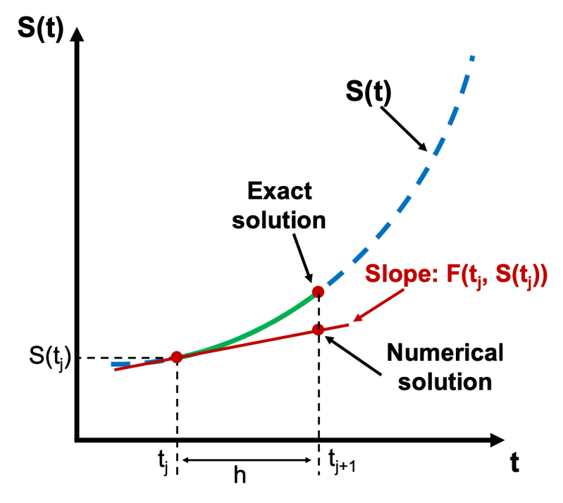
The method’s origins trace back to the 18th century, when Euler sought to translate continuous mathematical models into discrete, computable steps. At its core, Euler’s method approximates the trajectory of a dynamic system by advancing in small, linear increments—each step a tangent-line approximation of the true solution. This "step-and-repeat" philosophy mirrors how nature itself unfolds: one infinitesimal change at a time. Yet its power isn’t merely historical; it’s alive in modern simulations, from climate modeling to financial forecasting, where precision often demands trade-offs between speed and accuracy.
While today’s supercomputers wield high-order solvers, Euler’s method endures as both a pedagogical tool and a practical baseline. Its simplicity belies its role in calibrating more complex algorithms, serving as a sanity check in fields where computational resources are constrained. Whether you’re a student grappling with differential equations or a researcher optimizing numerical workflows, understanding this method reveals the raw mechanics of how mathematics meets the real world.
The Complete Overview of Eulers Method
Euler’s method is the archetypal numerical technique for solving ordinary differential equations (ODEs), a class of problems where the rate of change of a function is known, but the function itself remains elusive. Imagine tracking the trajectory of a projectile under gravity: the velocity at any point is a function of time, but calculating its exact position requires integrating this relationship. Here, Euler’s method steps in, breaking the problem into tiny, manageable segments where each step’s output becomes the next step’s input. This iterative process—often called Euler integration—transforms an intractable continuous problem into a series of linear approximations, each governed by the equation:\[ y_{n+1} = y_n + h \cdot f(t_n, y_n) \]
where \( h \) is the step size, \( f \) defines the differential equation, and \( y_n \) approximates the solution at step \( n \). The method’s elegance lies in its universality: it applies to any ODE, from population growth models to electrical circuit simulations, provided the equation is well-behaved.
Table of Contents
- The Complete Overview of Eulers Method
- Historical Background and Evolution
- Core Mechanisms: How It Works
- Key Benefits and Crucial Impact
- Major Advantages
- Comparative Analysis
- Future Trends and Innovations
- Conclusion
- Comprehensive FAQs
- Q: Why does Eulers method accumulate error over time?
- Q: Can Eulers method solve partial differential equations (PDEs)?
- Q: How does step size \( h \) affect the accuracy and stability of Eulers method?
- Q: What are some real-world applications where Eulers method is still used today?
- Q: How does the modified Euler method (or Heun’s method) improve upon the basic Euler approach?
Yet its simplicity is a double-edged sword. Euler’s method is prone to accumulating errors over successive steps—a phenomenon known as truncation error—which grows with larger step sizes or stiff equations (those with widely varying solution scales). This inherent instability forces practitioners to balance computational efficiency with accuracy, often requiring adaptive step-sizing or hybrid approaches. Despite these challenges, the method’s transparency makes it indispensable for debugging more opaque solvers and for teaching the fundamental principles of numerical stability and convergence.
Historical Background and Evolution
The seeds of Euler’s method were sown in the 1760s, when Leonhard Euler formalized the concept of numerical integration to solve Kepler’s equation—a critical problem in celestial mechanics. His work on planetary motion demanded a way to approximate solutions where analytical methods failed, leading to the first documented use of what we now recognize as the Euler step. The method’s early adoption in astronomy and ballistics underscored its practical utility, though its theoretical limitations remained unaddressed until the 19th century, when mathematicians like Carl Runge and Wilhelm Kutta refined it into higher-order schemes.The 20th century saw Euler’s method evolve alongside the rise of digital computing. As engineers and physicists tackled increasingly complex systems—from aerodynamics to quantum mechanics—the method’s computational demands became a bottleneck. This spurred innovations like the backward Euler method (for stiff equations) and predictor-corrector techniques, which borrowed Euler’s iterative framework while mitigating its errors. Today, Euler’s method is rarely used in isolation for production-grade simulations, yet its influence persists in hybrid algorithms (e.g., semi-implicit methods) and as a building block for more advanced solvers like the exponential integrators used in molecular dynamics.
Core Mechanisms: How It Works
At its heart, Euler’s method operates on two pillars: discretization and iteration. Discretization converts the continuous domain of an ODE into a finite grid of points, where the solution is approximated at each node. The iteration then marches forward step-by-step, using the derivative (slope) at the current point to estimate the next. For example, solving \( \frac{dy}{dt} = -ky \) (exponential decay) with initial condition \( y(0) = y_0 \) and step size \( h = 0.1 \) yields:\[ y_{n+1} = y_n + h \cdot (-k y_n) = y_n (1 - k h) \]
Each step’s error stems from replacing the true (curved) solution with a straight-line tangent—a local error that compounds globally. The method’s stability hinges on the step size \( h \): if \( h \) is too large, the approximation diverges; if too small, computational cost explodes. This trade-off is quantified by the local truncation error, which scales as \( O(h^2) \) for smooth problems, but deteriorates for nonlinear or oscillatory systems.
The method’s geometric interpretation is equally revealing. In phase space, each Euler step traces a polygonal path approximating the true trajectory. For stiff equations (e.g., \( \frac{dy}{dt} = \lambda y \) with \( |\lambda| \gg 1 \)), this path spirals outward unless \( h \) is impractically small—a flaw that necessitated the development of implicit methods like backward Euler. Yet in non-stiff systems, the method’s linear complexity (\( O(N) \) for \( N \) steps) and minimal memory requirements make it a staple for prototyping and educational demonstrations.
Key Benefits and Crucial Impact
Euler’s method may seem rudimentary, but its impact on numerical analysis is immeasurable. It democratized the solution of differential equations, allowing scientists to explore phenomena previously confined to theoretical abstraction. From predicting chemical reaction rates to simulating stock market trends, the method’s adaptability has made it a workhorse in interdisciplinary research. Its role in teaching is equally critical: by exposing students to the nuances of numerical stability, convergence, and error propagation, it fosters intuition that transcends specific algorithms.The method’s enduring relevance lies in its ability to serve as a "control" for more sophisticated techniques. When debugging a Runge-Kutta solver, for instance, comparing its output to an Euler approximation can reveal hidden instabilities. Similarly, in machine learning, Euler-like updates underpin gradient descent—a cornerstone of optimization. Even in finance, the Euler-Maruyama scheme extends the method to stochastic differential equations, bridging deterministic and probabilistic modeling.
> "Euler’s method is the canary in the coal mine of numerical analysis: its failures often signal deeper issues in problem formulation or algorithmic design." — Numerical Recipes (Press et al.)
Major Advantages
- Simplicity and Transparency: Requires only basic arithmetic and a single function evaluation per step, making it easy to implement and debug.
- Low Computational Overhead: Operates in \( O(N) \) time and space, ideal for real-time applications or resource-constrained environments.
- Universal Applicability: Works for any ODE, linear or nonlinear, provided the derivative \( f(t, y) \) is computable.
- Educational Value: Serves as the foundation for understanding higher-order methods, error analysis, and numerical stability.
- Hybrid Compatibility: Often used as a preliminary step in multi-step methods (e.g., Adams-Bashforth) or embedded in adaptive solvers.

Comparative Analysis
| Criteria | Euler’s Method | Runge-Kutta (RK4) |
|---|---|---|
| Order of Accuracy | First-order (\( O(h^2) \) local error) | Fourth-order (\( O(h^5) \) local error) |
| Stability | Conditionally stable; requires small \( h \) for stiff equations | More stable for non-stiff problems, but still limited |
| Computational Cost | 1 function evaluation per step | 4 function evaluations per step |
| Best Use Case | Quick prototyping, teaching, or when \( O(h) \) error is acceptable | High-accuracy simulations where cost is secondary |
Future Trends and Innovations
As computational power grows, Euler’s method is evolving beyond its traditional role. In machine learning, variants like the Neural Euler method integrate neural networks with differential solvers, enabling data-driven approximations of PDEs. Meanwhile, geometric integration techniques—inspired by Euler’s work—preserve qualitative properties (e.g., energy conservation) in long-time simulations, critical for climate modeling and astrophysics. The rise of quantum computing may also reshape numerical methods, with Euler-like algorithms adapted to simulate quantum dynamics on noisy intermediate-scale devices.Another frontier is adaptive mesh refinement, where Euler’s method dynamically adjusts step sizes based on local error estimates, merging its simplicity with modern efficiency. Hybrid approaches, such as combining Euler steps with machine-learned correctors, promise to retain the method’s interpretability while achieving RK4-like accuracy. As problems grow in complexity—from multi-scale biological systems to high-dimensional PDEs—Euler’s iterative philosophy will likely remain a guiding principle, albeit in increasingly sophisticated forms.

Conclusion
Euler’s method is more than a relic of numerical analysis; it is a living paradigm that embodies the tension between simplicity and power. Its ability to approximate solutions with minimal assumptions has made it a touchstone for generations of mathematicians and engineers. While modern solvers have surpassed it in accuracy, the method’s influence is undiminished, serving as both a benchmark and a springboard for innovation. In an era where computational models underpin everything from drug discovery to space exploration, understanding Euler’s method is to grasp the very essence of how mathematics translates into actionable insight.Yet its legacy extends beyond utility. Euler’s method teaches us that even the most basic tools can unlock profound discoveries—provided we wield them with curiosity and rigor. As numerical analysis continues to evolve, the principles it embodies—discretization, iteration, and the pursuit of approximate truth—will remain as relevant as ever.
Comprehensive FAQs
Q: Why does Eulers method accumulate error over time?
The error in Euler’s method arises because each step approximates the true solution with a tangent line, introducing a local truncation error. This error compounds globally due to the method’s first-order accuracy, causing the approximation to drift further from the exact solution as the number of steps increases. The total error after \( N \) steps scales as \( O(h) \), where \( h \) is the step size.
Q: Can Eulers method solve partial differential equations (PDEs)?
While Euler’s method is primarily designed for ordinary differential equations (ODEs), it can be extended to PDEs via method of lines, where spatial derivatives are discretized (e.g., using finite differences) and the resulting system of ODEs is solved with Euler steps. However, this approach is rarely used in practice due to its poor stability for multi-dimensional problems; higher-order methods like finite element or spectral methods are preferred.
Q: How does step size \( h \) affect the accuracy and stability of Eulers method?
The step size \( h \) is a critical parameter: smaller \( h \) improves accuracy (reducing truncation error) but increases computational cost. For stability, \( h \) must satisfy \( h < \frac{2}{\lambda} \) for linear problems \( \frac{dy}{dt} = \lambda y \) with \( \lambda > 0 \). In stiff equations (where \( \lambda \) is large), \( h \) must be impractically small, making implicit methods like backward Euler more suitable.
Q: What are some real-world applications where Eulers method is still used today?
Despite its limitations, Euler’s method remains practical in:
- Real-time systems (e.g., robotics, control theory) where speed outweighs precision.
- Monte Carlo simulations for stochastic processes (e.g., finance, physics).
- Initial guesses for iterative solvers in optimization problems.
- Educational demonstrations to illustrate numerical convergence.
Q: How does the modified Euler method (or Heun’s method) improve upon the basic Euler approach?
The modified Euler method (a second-order Runge-Kutta variant) improves accuracy by averaging two Euler steps: one forward and one backward. Given \( y_{n+1} = y_n + h f(t_n, y_n) \) (forward) and \( y_{n+1}^* = y_n + h f(t_{n+1}, y_{n+1}) \) (backward), the modified step is:
\[ y_{n+1} = y_n + \frac{h}{2} \left[ f(t_n, y_n) + f(t_{n+1}, y_{n+1}^*) \right]. \]
This reduces the local error to \( O(h^3) \), offering better precision for the same computational cost as basic Euler.
Leave a Comment
Comments are moderated before appearing. The data you submit is processed according to the Privacy Policy of Gouv.