How Euler’s Method Solves Differential Equations with Stunning Precision
Leonhard Euler’s name echoes through the annals of mathematics like a theorem carved in stone—yet his method for approximating solutions to differential equations remains as practical today as it was in the 18th century. While modern supercomputers crunch data at lightning speeds, the core principle behind Euler’s method endures: a simple, iterative approach that transforms complex continuous problems into manageable discrete steps. It’s not just a tool for academics; engineers use it to model projectile trajectories, economists apply it to simulate market dynamics, and physicists rely on it to approximate chaotic systems. The genius lies in its simplicity: given a starting point and a slope, Euler’s method marches forward in tiny increments, stitching together a path where exact solutions are elusive.
The method’s elegance is deceptive. At its heart, it’s a first-order approximation—crude by some standards, yet remarkably effective for problems where precision isn’t the sole priority. Its limitations are well-documented: errors accumulate with each step, and stability can falter for stiff equations. Yet these flaws don’t diminish its value. They force practitioners to think critically about trade-offs between accuracy and computational cost, a lesson as relevant in software optimization as it is in theoretical math. The method’s robustness in educational settings further cements its legacy, serving as the gateway through which students grasp the broader landscape of numerical analysis.
What makes Euler’s method truly fascinating is its adaptability. Whether applied to ordinary differential equations (ODEs) or partial differential equations (PDEs), the underlying philosophy remains unchanged: discretize, approximate, iterate. This universality has spawned countless variations—from the improved Euler method (Heun’s method) to Runge-Kutta schemes—each refining the original concept while preserving its foundational principles. The method’s ability to bridge theory and application ensures its place not just in textbooks, but in the toolkits of scientists and engineers worldwide.

The Complete Overview of Euler’s Method
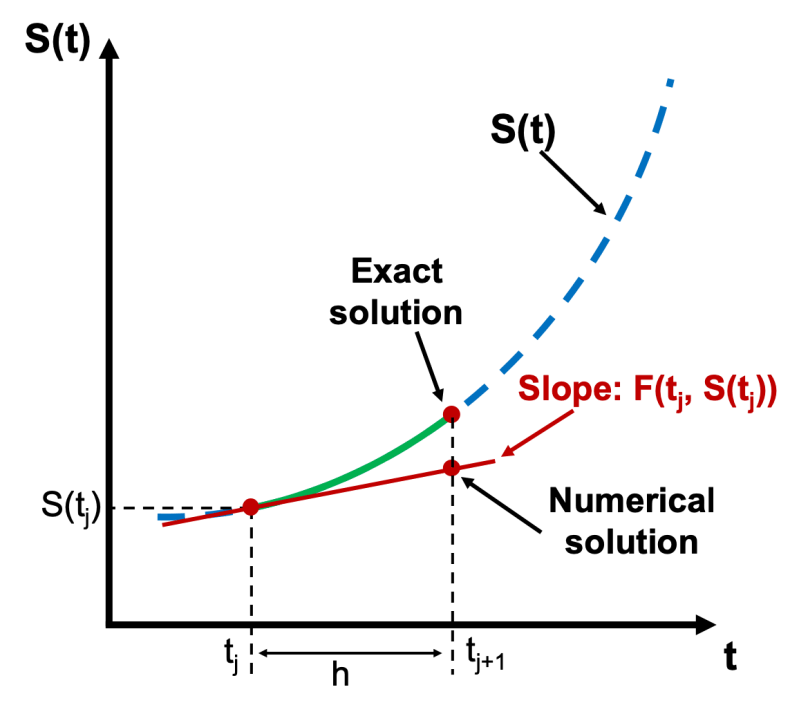
At its core, Euler’s method is a numerical technique designed to approximate solutions to initial value problems (IVPs) in differential equations. When an exact analytical solution is intractable—whether due to the equation’s complexity or the boundary conditions—Euler’s method provides a practical alternative. By breaking the problem into small, linear segments, it approximates the solution curve as a series of connected straight lines, each representing the tangent at a discrete point. This piecewise linear approximation is surprisingly effective for problems where high precision isn’t critical, or where computational resources are limited.The method’s simplicity belies its power. Given a differential equation of the form dy/dx = f(x, y) with an initial condition y(x₀) = y₀, Euler’s method computes subsequent points using the formula:
yₙ₊₁ = yₙ + h·f(xₙ, yₙ)
where h is the step size (Δx). Each iteration advances the solution by one step, using the slope at the current point to estimate the next. While this linear approximation introduces error, reducing h refines the result—though at the cost of increased computational effort. The trade-off between step size and accuracy is a central theme in numerical analysis, and Euler’s method serves as the prototypical example of this dilemma.
Historical Background and Evolution
The origins of Euler’s method trace back to the 18th century, when Leonhard Euler—one of history’s most prolific mathematicians—developed techniques to solve differential equations numerically. His work was motivated by the need to model physical phenomena where exact solutions were unattainable, such as the motion of celestial bodies or the behavior of fluids. Euler’s contributions laid the groundwork for what would later become numerical analysis, a field now indispensable in scientific computing.The method’s evolution is a testament to its adaptability. Early applications were limited by manual calculations, but the advent of mechanical computers in the 19th century and digital computers in the 20th century transformed its potential. By the mid-20th century, refinements like the predictor-corrector methods and Runge-Kutta techniques emerged, building upon Euler’s foundational ideas. Today, Euler’s method is often taught as the first step in understanding more sophisticated algorithms, serving as a scaffold for students before they tackle higher-order methods.
Core Mechanisms: How It Works
The mechanics of Euler’s method are straightforward yet profound. For a given differential equation dy/dx = f(x, y), the method proceeds as follows:1. Initialization: Start with an initial point (x₀, y₀) and a step size h.
2. Iteration: For each subsequent point xₙ₊₁ = xₙ + h, compute the slope f(xₙ, yₙ) at the current point.
3. Approximation: Use the slope to estimate the next y-value: yₙ₊₁ = yₙ + h·f(xₙ, yₙ).
4. Repeat: Continue until the desired endpoint is reached.
Table of Contents
- The Complete Overview of Euler’s Method
- Historical Background and Evolution
- Core Mechanisms: How It Works
- Key Benefits and Crucial Impact
- Major Advantages
- Comparative Analysis
- Future Trends and Innovations
- Conclusion
- Comprehensive FAQs
- Q: What is the primary limitation of Euler’s method?
- Q: How does step size h affect the accuracy of Euler’s method?
- Q: Can Euler’s method be used for partial differential equations (PDEs)?
- Q: What is the difference between Euler’s method and the improved Euler method?
- Q: Are there real-world applications where Euler’s method is the best choice?
- Q: How does Euler’s method relate to gradient descent in machine learning?
This process generates a sequence of points that approximate the true solution curve. The accuracy of the approximation depends on the step size h: smaller steps yield better results but require more computations. The method’s local truncation error (error per step) is O(h²), while the global truncation error (total error) is O(h), reflecting the cumulative nature of the approximation errors.
The method’s geometric interpretation is equally insightful. Each step corresponds to moving along the tangent line of the solution curve at the current point. While this linear approximation diverges from the true curve over time, the cumulative effect of many small steps can produce surprisingly accurate results for many practical applications.
Key Benefits and Crucial Impact
Euler’s method’s enduring relevance stems from its balance of simplicity and utility. It serves as an accessible introduction to numerical methods, demystifying the process of solving differential equations for students and practitioners alike. Its computational efficiency makes it ideal for real-time applications, such as control systems or simulations where speed is prioritized over absolute precision. Moreover, the method’s transparency—every step is mathematically explicit—enhances its pedagogical value, allowing users to debug and refine their approach with ease.Beyond its educational role, Euler’s method has practical applications across disciplines. In physics, it models trajectories in ballistics and orbital mechanics. Economists use it to simulate dynamic systems, such as population growth or financial markets. Even in machine learning, variants of Euler’s method appear in optimization algorithms, where gradient descent can be viewed as an iterative Euler-like update. The method’s versatility ensures its continued relevance in an era dominated by high-performance computing.
> "Euler’s method is not just a tool; it’s a lens through which we understand the interplay between approximation and reality. Its limitations reveal deeper truths about numerical stability and error propagation, shaping the development of more advanced techniques." — Numerical Analysis Textbook, 20th Edition
Major Advantages
- Simplicity: Requires minimal computational overhead, making it easy to implement and understand.
- Versatility: Applicable to a wide range of differential equations, from linear ODEs to simple PDEs.
- Educational Value: Serves as the foundational building block for more complex numerical methods.
- Real-Time Applicability: Suitable for systems where low-latency approximations are critical.
- Theoretical Insight: Highlights the trade-offs between step size, accuracy, and computational cost.
Comparative Analysis
While Euler’s method is a cornerstone of numerical analysis, other techniques offer improvements in accuracy and stability. Below is a comparison of key methods:| Method | Key Characteristics |
|---|---|
| Euler’s Method | First-order, simple, O(h) global error; prone to divergence for stiff equations. |
| Improved Euler (Heun’s Method) | Second-order, uses average slope for better accuracy; O(h²) global error. |
| Runge-Kutta (RK4) | Fourth-order, highly accurate; O(h⁴) global error but computationally intensive. |
| Predictor-Corrector (Adams-Bashforth) | Multi-step method; better stability for non-stiff problems but requires initial steps. |
Future Trends and Innovations
The future of Euler’s method lies in its integration with modern computational techniques. As machine learning and high-performance computing advance, hybrid approaches—combining Euler’s iterative simplicity with adaptive step sizes or neural network enhancements—are emerging. For instance, adaptive Euler methods dynamically adjust h to balance accuracy and efficiency, while stochastic Euler methods extend the technique to stochastic differential equations (SDEs), crucial in finance and quantum physics.Additionally, the rise of symbolic-numeric hybrid methods—where symbolic computation refines numerical approximations—could redefine Euler’s role. Imagine a system where Euler’s method provides an initial guess, which is then optimized using symbolic algebra or machine learning. Such innovations would preserve the method’s intuitive appeal while pushing its boundaries into domains previously deemed too complex.

Conclusion
Euler’s method remains a testament to the power of simplicity in mathematics. Its ability to transform intractable differential equations into manageable approximations has cemented its place in both theory and practice. While modern alternatives offer higher precision, Euler’s method endures as a fundamental tool, a bridge between abstract concepts and real-world applications. Its legacy is not just in its historical significance but in its continued relevance, proving that sometimes, the most elegant solutions are the ones that stand the test of time.As numerical analysis evolves, Euler’s method will likely persist as both a teaching tool and a practical algorithm, its principles embedded in more sophisticated techniques. The method’s ability to inspire curiosity—whether in a student’s first encounter with differential equations or an engineer’s quest for efficient simulations—ensures its survival in an ever-advancing field.
Comprehensive FAQs
Q: What is the primary limitation of Euler’s method?
A: The primary limitation is its global truncation error, which accumulates linearly with each step (O(h)). This makes it less accurate for long-term simulations compared to higher-order methods like Runge-Kutta. Additionally, it struggles with stiff equations, where small step sizes are required for stability, increasing computational cost.
Q: How does step size h affect the accuracy of Euler’s method?
A: A smaller h reduces the local truncation error per step, improving overall accuracy but requiring more iterations. Conversely, a larger h speeds up computation but increases cumulative error. The choice of h is often a trade-off between precision and performance, guided by heuristics or adaptive strategies.
Q: Can Euler’s method be used for partial differential equations (PDEs)?
A: While Euler’s method is primarily designed for ordinary differential equations (ODEs), it can be extended to parabolic PDEs (e.g., heat equation) via the method of lines, where spatial derivatives are discretized first, converting the PDE into a system of ODEs solvable by Euler’s method. However, it’s rarely used for hyperbolic or elliptic PDEs due to stability issues.
Q: What is the difference between Euler’s method and the improved Euler method?
A: The improved Euler method (Heun’s method) enhances accuracy by using the average slope between two points: it first computes a temporary step using Euler’s formula, then refines it by averaging the slopes at the start and end of the interval. This reduces the global error to O(h²), making it more precise than the basic Euler method.
Q: Are there real-world applications where Euler’s method is the best choice?
A: Yes. Euler’s method is often preferred in real-time systems where computational speed is critical, such as:
Q: How does Euler’s method relate to gradient descent in machine learning?
A: Gradient descent is mathematically equivalent to Euler’s method applied to optimization problems. In gradient descent, the update rule θₙ₊₁ = θₙ − η·∇J(θₙ) mirrors Euler’s method, where η (learning rate) plays the role of h, and ∇J(θₙ) is the "slope" (gradient). This connection underscores Euler’s method’s broader influence beyond differential equations.
Leave a Comment
Comments are moderated before appearing. The data you submit is processed according to the Privacy Policy of Gouv.