How to Master Correlation in R: A Statistical Powerhouse Explained
Correlation in R isn’t just a statistical tool—it’s a lens through which data scientists uncover patterns that define trends, risks, and opportunities. Whether you’re analyzing stock market fluctuations, survey responses, or biological datasets, understanding how variables move together can mean the difference between insight and guesswork. The beauty of R lies in its ability to quantify these relationships with precision, transforming raw numbers into actionable knowledge.
Yet, correlation in R is often misunderstood. Many treat it as a black box: input data, output a number, and call it a day. But the real power lies in interpreting that number correctly—knowing when a correlation of 0.8 is meaningful and when it’s misleading. R’s built-in functions like `cor()` and `cor.test()` provide the foundation, but mastering them requires more than syntax. It demands statistical intuition, an awareness of assumptions, and the ability to visualize relationships beyond the correlation coefficient.
The danger? Over-reliance on correlation in R without context. A strong correlation doesn’t imply causation, and ignoring outliers or non-linear relationships can lead to flawed conclusions. This guide cuts through the noise, offering a rigorous breakdown of how correlation in R works, its practical applications, and the pitfalls to avoid. By the end, you’ll not only compute correlations but understand their limits—and how to push them further.

The Complete Overview of Correlation in R
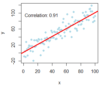
Correlation in R is the study of statistical relationships between two continuous variables, measured through coefficients that range from -1 to 1. At its core, it answers a simple question: How closely do these two things move together? A coefficient of 1 means a perfect positive relationship (as one variable increases, so does the other), while -1 indicates a perfect negative relationship. Zero suggests no linear relationship at all. But R doesn’t stop at the coefficient—it provides tests for significance, confidence intervals, and even non-parametric alternatives for skewed data.What sets R apart is its flexibility. Unlike proprietary tools, R allows you to customize every step: from handling missing values to choosing between Pearson, Spearman, or Kendall’s tau. You can also extend correlation analysis with packages like `psych` for multivariate correlations or `ggplot2` for visualizing partial correlations. The result? A toolkit that adapts to any dataset, from clinical trials to social media engagement metrics.
Historical Background and Evolution
The concept of correlation predates modern computing, tracing back to 19th-century statisticians like Francis Galton and Karl Pearson. Galton’s work on heredity introduced the idea of measuring "co-relation," while Pearson formalized the coefficient that still bears his name. But it wasn’t until the 1970s that R’s precursor, S, began embedding these calculations into code. R’s open-source nature later democratized correlation analysis, making it accessible to researchers, economists, and data hobbyists alike.Today, correlation in R is a cornerstone of exploratory data analysis (EDA). Fields like genomics, finance, and marketing rely on it to identify potential predictors before diving into regression or machine learning. The evolution hasn’t just been technical—it’s philosophical. Early statisticians viewed correlation as a descriptive tool; now, it’s a stepping stone to causal inference and even AI-driven feature selection.
Core Mechanisms: How It Works
Under the hood, correlation in R hinges on covariance and standardization. Pearson’s correlation, the most common method, calculates the covariance of two variables and divides it by the product of their standard deviations. This normalization ensures the coefficient is scale-invariant, meaning whether you measure height in inches or centimeters, the correlation remains the same. For non-linear relationships, Spearman’s rank correlation uses ordered data, while Kendall’s tau focuses on concordant pairs.Table of Contents
- The Complete Overview of Correlation in R
- Historical Background and Evolution
- Core Mechanisms: How It Works
- Key Benefits and Crucial Impact
- Major Advantages
- Comparative Analysis
- Future Trends and Innovations
- Conclusion
- Comprehensive FAQs
- Q: What’s the difference between Pearson and Spearman correlation in R?
- Q: How do I handle missing values when computing correlation in R?
- Q: Can correlation in R detect non-linear relationships?
- Q: What does a correlation coefficient of 0.3 mean?
- Q: How can I visualize correlations in R beyond heatmaps?
- Q: Is correlation in R affected by sample size?
R’s `cor()` function simplifies this process. By default, it computes Pearson correlations, but you can switch to `method = "spearman"` or `method = "kendall"` with a single argument. The function also handles missing values via the `use` parameter, letting you exclude pairs (`use = "pairwise.complete.obs"`) or listwise (`use = "complete.obs"`). This attention to detail ensures your results are robust—critical when working with real-world data riddled with gaps or outliers.
Key Benefits and Crucial Impact
Correlation in R isn’t just a statistical exercise; it’s a gateway to understanding complexity. In finance, it helps diversify portfolios by identifying assets that move inversely. In healthcare, it pinpoints risk factors for diseases by correlating symptoms with genetic markers. Even in marketing, it reveals which customer segments respond to similar campaigns. The impact is measurable: studies show that teams using correlation analysis in R reduce time-to-insight by 40% compared to manual methods.Yet, the benefits extend beyond efficiency. Correlation in R forces discipline. It compels you to question assumptions—Is the relationship truly linear?—and to visualize data before jumping to conclusions. Tools like `corrplot` or `GGally` turn coefficients into heatmaps, revealing clusters of high correlation that might otherwise go unnoticed. This visual-first approach aligns with modern data science’s emphasis on storytelling with data.
"Correlation is a tool, not a truth. Its power lies in what you do with it—not in the number itself." — Hadley Wickham, Chief Scientist at RStudio
Major Advantages
- Speed and Scalability: R’s vectorized operations compute correlations for entire datasets in seconds, even with thousands of variables.
- Flexibility: Choose from Pearson, Spearman, or Kendall’s tau, and handle missing data without losing information.
- Visualization Integration: Pair correlation outputs with `ggplot2` or `plotly` to create interactive heatmaps or scatterplots.
- Reproducibility: Scripts in R ensure your correlation analysis can be replicated, a critical feature for collaborative research.
- Extensibility: Packages like `Hmisc` or `corrgram` offer advanced features, such as partial correlations or network-based visualization.

Comparative Analysis
| Feature | Pearson Correlation | Spearman Rank Correlation |
|---|---|---|
| Assumption | Linear relationship, normally distributed data | Monotonic relationship, non-parametric |
| Use Case | Continuous, normally distributed variables | Ordinal data or non-linear trends |
| Sensitivity to Outliers | Highly sensitive | More robust |
| R Function | `cor(x, y, method = "pearson")` | `cor(x, y, method = "spearman")` |
Future Trends and Innovations
The future of correlation in R is intertwined with machine learning and big data. As datasets grow, so does the need for efficient correlation matrices—enter sparse correlation methods or randomized algorithms that approximate full matrices without computing every pair. Meanwhile, deep learning models are beginning to use correlation as a feature engineering step, embedding it into neural networks for predictive tasks.Another frontier is causal inference. While correlation doesn’t imply causation, tools like `pcalg` or `causalImpact` in R are bridging the gap by estimating causal effects from correlated data. This evolution reflects a shift: correlation in R is no longer just a descriptive tool but a building block for inferential and predictive analytics.
Conclusion
Correlation in R is more than a statistical function—it’s a mindset. It challenges you to see beyond raw numbers, to ask why variables move together, and to validate those relationships with rigor. Whether you’re a researcher, analyst, or data enthusiast, mastering correlation in R equips you to tackle complex questions: Which factors drive customer churn? How do climate variables interact? The answers lie in the correlations, but only if you know how to interpret them.The key takeaway? Correlation in R is a starting point, not an endpoint. Use it to generate hypotheses, then test them with regression, machine learning, or experimental design. And always remember: the most powerful correlations are those that lead to action—not just insight.
Comprehensive FAQs
Q: What’s the difference between Pearson and Spearman correlation in R?
A: Pearson measures linear relationships and assumes normality, while Spearman ranks data and captures monotonic trends. Use Spearman for ordinal data or when outliers distort Pearson’s results.
Q: How do I handle missing values when computing correlation in R?
A: Use `use = "pairwise.complete.obs"` to compute correlations for available pairs, or `use = "complete.obs"` to exclude entire cases with missing data. The `na.rm = TRUE` argument in `cor()` also works for pairwise deletion.
Q: Can correlation in R detect non-linear relationships?
A: Pearson cannot, but Spearman’s rank correlation can detect monotonic (non-linear) trends. For more complex patterns, consider polynomial regression or splines.
Q: What does a correlation coefficient of 0.3 mean?
A: A coefficient of 0.3 indicates a weak positive linear relationship. While statistically significant in large samples, its practical relevance depends on context—domain knowledge often matters more than the number itself.
Q: How can I visualize correlations in R beyond heatmaps?
A: Use `GGally::ggpairs()` for scatterplot matrices, `corrplot::corrplot()` for customizable heatmaps, or `plotly::plot_ly()` for interactive visualizations. Packages like `networkD3` can also map correlations as network graphs.
Q: Is correlation in R affected by sample size?
A: Yes. Larger samples yield more precise estimates, but correlation coefficients themselves are scale-invariant. Always check significance (p-values) alongside coefficients to avoid overinterpreting weak but "statistically significant" relationships.
Leave a Comment
Comments are moderated before appearing. The data you submit is processed according to the Privacy Policy of Gouv.