Insertion Sort Best Case: When Algorithms Shine Brightest
Insertion sort is often dismissed as a "simple" algorithm—one relegated to educational examples or trivial datasets. Yet, its elegance lies in a paradox: what many overlook as a limitation becomes its greatest strength under the right conditions. When data arrives already ordered, insertion sort doesn’t just perform—it excels. This is the insertion sort best case, a scenario where the algorithm’s linear time complexity (O(n)) becomes its defining characteristic, outpacing even more celebrated methods in specific contexts.
The distinction between worst-case and best-case behavior in insertion sort isn’t merely academic. It reflects a deeper truth about algorithmic design: efficiency isn’t static. It’s dynamic, shaped by input characteristics. While average-case performance often dominates discussions, the insertion sort best case reveals how preprocessing, data locality, or even human behavior (e.g., user-generated sorted lists) can turn an "inefficient" algorithm into a high-performance tool. Understanding this isn’t just about optimizing code—it’s about recognizing when simplicity aligns with speed.

The Complete Overview of Insertion Sort’s Best-Case Performance
Insertion sort’s reputation as a "slow" algorithm stems from its quadratic worst-case time complexity (O(n²)), where each new element may require shifting through the entire sorted portion of the array. However, this narrative ignores the algorithm’s insertion sort best case, where the input is pre-sorted or nearly sorted. In such scenarios, the algorithm reduces to a series of O(1) comparisons and minimal swaps, achieving O(n) time complexity—identical to the best-case performance of merge sort or quicksort. This duality underscores why insertion sort remains relevant in niche applications, from embedded systems to adaptive sorting pipelines.The key to unlocking insertion sort’s best-case efficiency lies in its incremental nature. Unlike divide-and-conquer algorithms that recursively partition data, insertion sort builds a sorted array one element at a time. When each new element is already in its correct position relative to the sorted subarray, the algorithm skips unnecessary comparisons and shifts. This behavior isn’t just theoretical; it’s observable in real-world data streams where elements arrive in ascending or descending order, such as sensor readings, log files, or financial transactions processed in chronological sequence.
Historical Background and Evolution
Insertion sort’s origins trace back to the 1940s, when early computing pioneers like John von Neumann and Herman Goldstine documented it in foundational works on sorting networks. At the time, memory constraints and hardware limitations made insertion sort an attractive choice—its in-place nature (requiring only O(1) additional space) and adaptive behavior aligned with the era’s computational realities. However, as computers grew more powerful, the algorithm’s quadratic worst-case performance became a liability, pushing it to the periphery in favor of O(n log n) alternatives like quicksort or mergesort.Yet, the insertion sort best case persisted as a cornerstone of adaptive sorting techniques. In the 1970s, Donald Knuth highlighted its efficiency for partially sorted data in The Art of Computer Programming, cementing its role in hybrid algorithms. Modern adaptations, such as Timsort (Python’s built-in sort), leverage insertion sort’s best-case behavior for small or nearly ordered subarrays, combining it with merge sort to achieve optimal performance across diverse inputs. This evolution reveals a critical insight: the insertion sort best case isn’t a relic of the past—it’s a testament to the algorithm’s resilience in specialized domains.
Core Mechanisms: How It Works
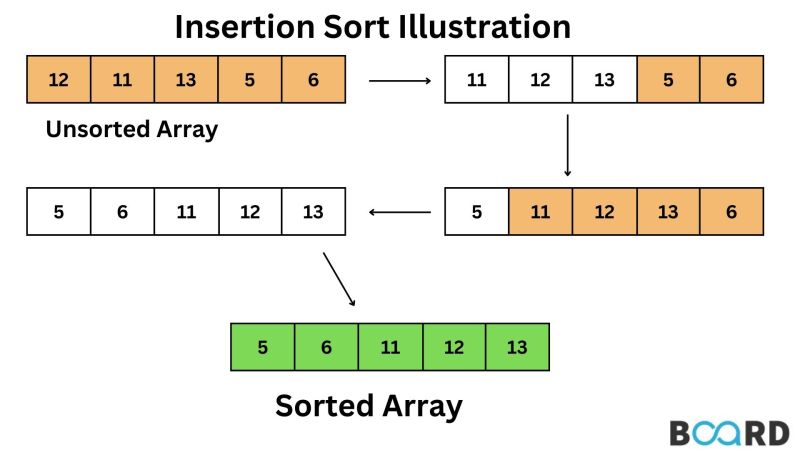
At its core, insertion sort operates by maintaining a sorted subarray and iteratively inserting each new element into its correct position. The algorithm’s pseudocode is deceptively simple:```
for i from 1 to n-1:
key = array[i]
j = i - 1
while j >= 0 and array[j] > key:
array[j + 1] = array[j]
j = j - 1
array[j + 1] = key
```
In the insertion sort best case, the `while` loop never executes because `array[j] <= key` for all `j`. Each element is already positioned correctly, reducing the inner loop to a single assignment. This linear progression—where comparisons and shifts are minimized—is what transforms insertion sort from a quadratic algorithm into an O(n) powerhouse.
The efficiency gain stems from two factors: data locality and adaptive comparisons. Locality ensures that memory accesses are contiguous, reducing cache misses, while adaptive comparisons exploit the input’s inherent order. For example, sorting a list `[1, 2, 3, 4]` requires only four comparisons (one per element) and zero shifts, achieving the theoretical minimum. This behavior is particularly advantageous in scenarios where preprocessing guarantees sortedness, such as merging two pre-sorted arrays or handling streaming data with known monotonicity.
Key Benefits and Crucial Impact
The insertion sort best case isn’t just an academic curiosity—it’s a practical advantage in systems where input characteristics are predictable. Unlike algorithms that assume randomness, insertion sort thrives on structure. This adaptability makes it ideal for real-time applications where data arrives in a controlled order, such as:Table of Contents
- The Complete Overview of Insertion Sort’s Best-Case Performance
- Historical Background and Evolution
- Core Mechanisms: How It Works
- Key Benefits and Crucial Impact
- Major Advantages
- Comparative Analysis
- Future Trends and Innovations
- Conclusion
- Comprehensive FAQs
- Q: What defines the "best case" for insertion sort?
- Q: How does insertion sort’s best case compare to its average case?
- Q: Can insertion sort be optimized further in its best case?
- Q: Where is insertion sort’s best-case behavior most useful?
- Q: Why isn’t insertion sort used more widely despite its best-case efficiency?
- Q: How does insertion sort’s best case relate to hybrid algorithms like Timsort?
The algorithm’s simplicity also translates to lower constant factors. While O(n log n) algorithms like quicksort may outperform insertion sort in average cases, the insertion sort best case often requires fewer operations due to reduced branching and memory access patterns. This efficiency isn’t just about speed—it’s about predictability. In environments where worst-case scenarios are unacceptable (e.g., real-time control systems), insertion sort’s best-case behavior provides a reliable performance floor.
"Insertion sort is a reminder that the most elegant solutions often lie in simplicity, not complexity. Its best-case performance is a masterclass in how algorithms can adapt to their inputs rather than fight them." — Donald Knuth, The Art of Computer Programming
Major Advantages
- Linear Time Complexity (O(n)): In the insertion sort best case, the algorithm achieves optimal time complexity, matching the lower bound for comparison-based sorting.
- In-Place Execution: Requires only O(1) additional space, making it ideal for memory-constrained environments where auxiliary storage is prohibitive.
- Adaptive Nature: Performance improves as input order improves, unlike algorithms with fixed complexity regardless of input structure.
- Low Overhead: Minimal branching and memory operations in the best case result in fewer cache misses and faster execution than many O(n log n) alternatives.
- Stability: Preserves the relative order of equal elements, a critical feature in applications like database sorting where ties must be handled predictably.
Comparative Analysis
While insertion sort excels in the insertion sort best case, its performance diverges sharply in other scenarios. Below is a comparison with other sorting algorithms under ideal and worst-case conditions:| Algorithm | Best Case / Worst Case Complexity |
|---|---|
| Insertion Sort | O(n) / O(n²) |
| Merge Sort | O(n log n) / O(n log n) |
| Quicksort | O(n log n) / O(n²) |
| Timsort (Hybrid) | O(n) / O(n log n) |
Future Trends and Innovations
The insertion sort best case is poised to regain relevance in two emerging domains. First, adaptive machine learning models increasingly rely on sorted or partially sorted data. Algorithms like Timsort, which combine insertion sort with merge sort, are being optimized for GPU acceleration, where insertion sort’s locality benefits from parallel memory access patterns. Second, quantum computing research is exploring insertion sort’s potential as a hybrid classical-quantum algorithm, where its adaptive nature could reduce qubit operations for pre-sorted inputs.Another frontier is real-time streaming systems, where data arrives in temporal order. Insertion sort’s O(n) best-case performance aligns with the needs of applications like fraud detection or IoT sensor networks, where latency is critical. Future innovations may integrate insertion sort with approximate sorting techniques, trading off absolute correctness for speed in scenarios where near-sorted outputs are sufficient.
Conclusion
Insertion sort’s best-case scenario is a microcosm of algorithmic design: what appears as a limitation can become an asset when leveraged correctly. Its linear efficiency for pre-sorted data isn’t a fluke—it’s a deliberate adaptation to real-world constraints, from memory limitations to structured input streams. While modern algorithms dominate general-purpose sorting, insertion sort’s niche advantages ensure its survival in specialized contexts, particularly where adaptability and simplicity are prized over raw speed.The lesson for practitioners is clear: algorithm selection isn’t about absolute metrics but contextual fit. The insertion sort best case serves as a reminder that the most effective tools are those that align with the problem’s inherent structure. As data patterns evolve—whether through AI-generated datasets or real-time analytics—the principles underlying insertion sort’s efficiency will continue to inspire hybrid and adaptive sorting strategies.
Comprehensive FAQs
Q: What defines the "best case" for insertion sort?
The insertion sort best case occurs when the input array is already sorted in ascending or descending order. In this scenario, each element requires only a single comparison (to confirm its correct position) and no shifts, resulting in O(n) time complexity.
Q: How does insertion sort’s best case compare to its average case?
In the average case, insertion sort has O(n²) time complexity due to random data distributions requiring multiple comparisons and shifts per element. However, the insertion sort best case achieves O(n), making it asymptotically faster than the average case of O(n log n) algorithms like merge sort or quicksort.
Q: Can insertion sort be optimized further in its best case?
Yes. Techniques like binary search insertion sort (using binary search to find the insertion point) reduce comparisons to O(log n) per element, though shifts remain O(n). This hybrid approach maintains O(n) best-case time while improving average-case performance for nearly sorted data.
Q: Where is insertion sort’s best-case behavior most useful?
The insertion sort best case is particularly valuable in:
Q: Why isn’t insertion sort used more widely despite its best-case efficiency?
Insertion sort’s quadratic worst-case performance (O(n²)) makes it impractical for large, randomly ordered datasets. Modern algorithms like Timsort or quicksort (with optimizations) dominate general-purpose sorting by offering consistent O(n log n) performance, while insertion sort’s advantages are confined to specific, predictable input scenarios.
Q: How does insertion sort’s best case relate to hybrid algorithms like Timsort?
Hybrid algorithms like Timsort exploit insertion sort’s best-case efficiency for small or nearly sorted subarrays. By combining insertion sort with merge sort, Timsort achieves O(n) best-case performance while maintaining O(n log n) average-case complexity—a balance that makes it Python’s default sorting algorithm.
Leave a Comment
Comments are moderated before appearing. The data you submit is processed according to the Privacy Policy of Gouv.