How the p value formula reshapes modern hypothesis testing
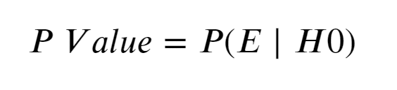
The p value formula isn’t just a mathematical tool—it’s the silent arbiter of scientific credibility. When researchers declare a drug effective, a political trend significant, or a machine learning model reliable, they’re implicitly relying on this probabilistic threshold. Yet its interpretation remains one of the most contentious debates in modern statistics. The formula itself, derived from the cumulative distribution function of the test statistic under the null hypothesis, seems straightforward: p = P(T ≥ t₀ | H₀), where t₀ is the observed test statistic. But the nuances—from Type I error inflation to Bayesian critiques—reveal a system far more complex than its surface-level application suggests.
Critics argue the p value formula has been weaponized, with journals favoring "statistically significant" results (p < 0.05) over nuanced effect sizes. The replication crisis in psychology and medicine traces back to over-reliance on this binary metric. Meanwhile, fields like genomics and high-energy physics have adopted stricter thresholds (e.g., p < 1e-8) to combat false discoveries. The formula’s flexibility is its strength—and its Achilles’ heel. Whether you’re validating a clinical trial or tuning a recommendation algorithm, understanding how the p value formula interacts with sample size, effect magnitude, and multiple testing is non-negotiable.
At its core, the p value formula bridges raw data and scientific claims. It quantifies the probability of observing extreme results if the null hypothesis were true—a counterintuitive but powerful framework. Yet its limitations demand context: it doesn’t measure evidence for the alternative hypothesis, nor does it account for prior probabilities. The formula’s evolution, from Fisher’s early work to modern corrections like Bonferroni or false discovery rate (FDR), reflects an ongoing dialogue between rigor and practicality.

The Complete Overview of the p Value Formula
The p value formula serves as the linchpin of frequentist statistics, providing a standardized way to evaluate evidence against a null hypothesis. Its mathematical foundation lies in the distribution of a test statistic (e.g., t-score, chi-square, or z-score) under the assumption that the null is true. For a two-tailed test, the formula is expressed as:p = 2 × min(P(T ≥ |t₀|), P(T ≤ -|t₀|)) where T follows the relevant sampling distribution (e.g., normal, t, or F). This symmetry accounts for deviations in either direction, ensuring robustness against directional bias. The choice of test statistic depends on the data type: means (t-test), proportions (z-test), or categorical associations (chi-square). Even in non-parametric contexts, permutations or bootstrapping can approximate the p value formula empirically.
The formula’s power stems from its generality, but its application requires careful consideration of assumptions. For instance, a t-test assumes normality and homogeneity of variance, while a chi-square test demands expected frequencies >5. Violations can inflate Type I errors, leading to false positives. Modern software automates these calculations, but understanding the underlying mechanics—how sample size affects precision, how effect size influences detectability—remains critical. The p value formula isn’t a standalone answer; it’s a gateway to deeper questions about study design, power analysis, and the trade-offs between sensitivity and specificity.
Historical Background and Evolution
The p value formula emerged from the early 20th century’s statistical revolution, spearheaded by Ronald Fisher and Jerzy Neyman. Fisher, in Statistical Methods for Research Workers (1925), introduced the concept as a "probability of error" when rejecting the null, though he initially resisted the 0.05 threshold as arbitrary. Neyman and Pearson later formalized hypothesis testing as a decision framework, framing the p value as part of a broader Type I/II error trade-off. Their 1933 paper laid the groundwork for the Neyman-Pearson lemma, which optimizes test power for a given significance level—a direct consequence of the p value formula’s structure.The 1950s and 60s saw the formula’s institutionalization in medical and social sciences, often divorced from its probabilistic nuances. By the 1990s, critiques from statisticians like Stephen Senn and David Salsburg exposed its misapplication: p-values were being conflated with "proof," and multiple testing was ignored. The 2016 Nature "reproducibility crisis" papers forced a reckoning, leading to initiatives like the American Statistical Association’s 2016 statement on p-values, which emphasized effect sizes, confidence intervals, and prior evidence. Today, the p value formula endures not as an infallible rule but as a tool within a broader inferential toolkit.
Core Mechanisms: How It Works
The p value formula operates by comparing the observed test statistic (t₀) to the distribution of possible values under the null hypothesis. For a one-sample t-test, for example:1. Compute the sample mean (x̄) and standard error (SE).
2. Calculate the t-statistic: t₀ = (x̄ - μ₀) / SE, where μ₀ is the null-hypothesized mean.
3. The p value is the area under the t-distribution’s tails beyond |t₀|.
Table of Contents
- The Complete Overview of the p Value Formula
- Historical Background and Evolution
- Core Mechanisms: How It Works
- Key Benefits and Crucial Impact
- Major Advantages
- Comparative Analysis
- Future Trends and Innovations
- Conclusion
- Comprehensive FAQs
- Q: How does sample size affect the p value formula?
- Q: Can the p value formula distinguish between strong and weak evidence?
- Q: Why do some fields use stricter p-value thresholds (e.g., p < 1e-8)?
- Q: How does the p value formula interact with multiple testing?
- Q: What are the ethical implications of misusing the p value formula?
- Q: Are there alternatives to the p value formula?
This process assumes the null is true, making the p value a conditional probability—not a measure of the null’s plausibility. For instance, a p = 0.04 means there’s a 4% chance of observing data as extreme as t₀ if the null were correct. Crucially, it doesn’t imply a 96% chance the null is false. The formula’s sensitivity to sample size (n) is critical: larger n shrinks the standard error, increasing test power and often yielding "significant" results even for trivial effects—a phenomenon known as "statistical significance ≠ practical significance."
Key Benefits and Crucial Impact
The p value formula’s enduring relevance lies in its ability to standardize decision-making across disciplines. From pharmaceutical trials to cosmological data, it provides a common language for evaluating evidence. Its binary output (significant/non-significant) simplifies complex judgments, though this very clarity has fueled its misuse. The formula’s adaptability—through permutations, Monte Carlo simulations, or exact tests—also makes it versatile for non-normal or small-sample data. Without it, fields like genomics (where p < 1e-8 thresholds are common) or climate science (requiring multi-variable adjustments) would lack a framework to control false discoveries.Yet the formula’s impact extends beyond academia. Regulatory bodies (e.g., FDA, EMA) rely on p-values to approve drugs, while courts use them to assess forensic evidence. The 2009 Daubert v. Merrell Dow ruling even cited p-values as a benchmark for scientific validity. This institutional trust underscores the formula’s role as a gatekeeper of credibility—though its limitations, such as ignoring prior probabilities or effect sizes, have spurred alternatives like Bayesian methods or likelihood ratios.
"Significance testing is a very peculiar business. It is not a test of a hypothesis but a test of a hypothesis against a standard of error. The p-value is not the probability that the null hypothesis is true; it is the probability of the data given the null hypothesis." — Stephen Senn, Statistical Thinking in Modern Drug Development
Major Advantages
- Standardization: The p value formula provides a universal metric for comparing results across studies, enabling meta-analyses and systematic reviews.
- Decision Framework: It offers a clear threshold (e.g., α = 0.05) to balance Type I/II errors, crucial for high-stakes fields like medicine or aerospace.
- Flexibility: Adaptable to parametric (t-tests, ANOVA) and non-parametric (permutation tests) methods, making it suitable for diverse data types.
- Software Integration: Automated in R, Python (SciPy), and SPSS, reducing manual calculation errors and democratizing access.
- Regulatory Alignment: Institutionalized in guidelines (e.g., ICH-E9 for clinical trials), ensuring consistency in evidence evaluation.

Comparative Analysis
| Metric | p Value Formula | Bayesian Approach |
|---|---|---|
| Probabilistic Interpretation | P(Data | H₀); conditional on null | P(H₀ | Data); updates prior beliefs |
| Key Limitation | Ignores prior evidence; binary outcome | Requires subjective priors; computationally intensive |
| Use Case Strength | Exploratory research, large samples | Small samples, sequential testing |
| Threshold Example | p < 0.05 (arbitrary but conventional) | BF₀₁ > 3 (evidence ratio) |
Future Trends and Innovations
The p value formula’s future hinges on two competing forces: its entrenched utility and the rise of alternatives. Bayesian methods, with their emphasis on prior probabilities and posterior distributions, are gaining traction in fields like personalized medicine and AI, where p-values’ binary nature is inadequate. However, the formula’s simplicity and computational efficiency ensure its persistence, particularly in regulatory contexts. Innovations like the local false discovery rate (efron2007) or p-value adjustment methods (e.g., Benjamini-Hochberg) are refining its application in high-dimensional data (e.g., genomics). Meanwhile, the reproducibility crisis may accelerate shifts toward pre-registration, effect sizes, and multi-method validation—positioning the p value formula as one tool among many rather than the sole arbiter of truth.Emerging fields like quantum computing and complex systems may also redefine statistical inference. For instance, Bayesian neural networks already incorporate probabilistic priors, challenging the p value’s dominance. Yet, the formula’s role in hypothesis testing remains unmatched for its interpretability and speed. The challenge ahead is not to abandon it but to contextualize it within a broader framework—one that acknowledges its strengths while mitigating its pitfalls through transparency, replication, and interdisciplinary collaboration.
Conclusion
The p value formula is more than a statistical artifact; it’s a cultural artifact of scientific progress. Its history mirrors the evolution of evidence-based reasoning, from Fisher’s inductive leaps to today’s data-driven skepticism. While critiques abound—from its arbitrary thresholds to its failure to quantify evidence—the formula’s resilience stems from its role as a gatekeeper. It doesn’t prove anything, but it does ask the right questions: How likely is this result if the null holds? In an era of big data and algorithmic decision-making, those questions are more urgent than ever.Yet the formula’s future depends on its users. Blind adherence risks perpetuating the replication crisis; thoughtful integration with effect sizes, Bayesian methods, and domain knowledge can elevate it from a checklist item to a cornerstone of rigorous inquiry. The p value formula will endure, but its legacy will be defined by how we wield it—not as an end, but as a means to deeper understanding.
Comprehensive FAQs
Q: How does sample size affect the p value formula?
The p value formula is inversely related to sample size (n). Larger n reduces the standard error, increasing the test statistic’s magnitude and thus the likelihood of achieving significance (lower p). This can lead to "statistically significant" but trivial effects—a phenomenon called overfitting to noise. Researchers must balance n with effect size and power analysis to avoid misleading conclusions.
Q: Can the p value formula distinguish between strong and weak evidence?
No. The p value formula only quantifies the probability of observing data as extreme as the sample, given the null. A p = 0.04 doesn’t indicate "strong" evidence—it merely suggests the data are inconsistent with the null at the 5% level. Strength of evidence requires additional metrics, such as effect sizes (Cohen’s d), confidence intervals, or Bayesian posterior probabilities.
Q: Why do some fields use stricter p-value thresholds (e.g., p < 1e-8)?
Fields like genomics or particle physics use ultra-strict thresholds (e.g., p < 1e-8) to control the family-wise error rate (FWER) when testing millions of hypotheses simultaneously. Without adjustments, the probability of at least one false positive (Type I error) becomes unacceptably high. Methods like Bonferroni correction or false discovery rate (FDR) control address this, but they require careful calibration based on the number of tests.
Q: How does the p value formula interact with multiple testing?
Multiple testing inflates the chance of false positives. For m independent tests, the expected number of false positives at α = 0.05 is m × 0.05. Solutions include:
- Bonferroni correction: Divide α by m (conservative but simple).
- False Discovery Rate (FDR): Controls the expected proportion of false positives (e.g., Benjamini-Hochberg procedure).
- Holm-Bonferroni: A step-down method balancing power and error control.
Q: What are the ethical implications of misusing the p value formula?
Misuse—such as p-hacking (selecting analyses post-hoc to achieve significance) or HARKing (hypothesizing after results are known)—undermines scientific integrity. Ethical risks include:
- Wasted resources (e.g., funding failed replications).
- Public distrust (e.g., retracted studies like Begley & Ellis (2012)).
- Policy harm (e.g., approving ineffective drugs based on inflated p-values).
Q: Are there alternatives to the p value formula?
Yes. Key alternatives include:
- Bayesian Methods: Provide posterior probabilities (e.g., Bayes factors) and incorporate prior knowledge.
- Effect Sizes: Metrics like Cohen’s d or Hedges’ g quantify practical significance independent of sample size.
- Likelihood Ratios: Compare the likelihood of data under two hypotheses without arbitrary thresholds.
- Prediction Intervals: Focus on future data uncertainty rather than hypothesis testing.
Leave a Comment
Comments are moderated before appearing. The data you submit is processed according to the Privacy Policy of Gouv.