How Left Join Transforms Data Queries—The Definitive Breakdown
The left join is one of the most underappreciated yet indispensable tools in database management. While inner joins filter results to only matching rows, a left join ensures every record from the left table appears—even if no corresponding match exists in the right. This subtle distinction can mean the difference between a report that reveals gaps in customer data and one that obscures them entirely. Developers and analysts often overlook its nuanced behavior, treating it as a mere alternative to inner joins without understanding its broader implications for data integrity and business intelligence.
Consider an e-commerce platform where product listings (left table) need to be merged with inventory status (right table). A naive inner join would exclude products with zero stock, hiding critical insights about discontinued items. A left join, however, preserves all products while flagging those without inventory—transforming a simple query into a strategic decision-making tool. The operation’s elegance lies in its balance: it retains completeness without sacrificing performance, provided it’s implemented correctly.
Yet for all its utility, the left join remains a source of confusion. Many practitioners conflate it with outer joins or misapply it in scenarios where a different join type would be more efficient. The distinction between a left join and a left outer join—though technically redundant in most SQL dialects—exposes deeper questions about how databases handle NULL values and implicit conversions. Mastering this operation isn’t just about syntax; it’s about recognizing when to leverage its strengths and when to avoid its pitfalls.
The Complete Overview of Left Join
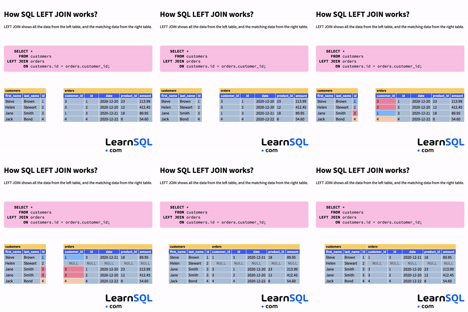
A left join is a relational database operation that combines rows from two tables based on a related column, with the defining characteristic that every row from the left (or primary) table is included in the result set, regardless of whether matches exist in the right (or secondary) table. This behavior contrasts sharply with inner joins, which return only rows where both tables have corresponding values. The left join’s ability to preserve all left-table records makes it indispensable for scenarios requiring comprehensive data retention, such as audits, inventory tracking, or customer segmentation.
The operation’s name stems from its directional nature: the "left" designation refers to the table positioned first in the join clause (e.g., `FROM table1 LEFT JOIN table2`). While some SQL dialects allow alternative syntax like `LEFT OUTER JOIN`, the core functionality remains identical. The key innovation lies in how it handles non-matching rows—by padding them with NULL values for columns from the right table—thereby maintaining referential integrity while accommodating missing data. This duality of inclusion and NULL handling is what distinguishes it from other join types.
Historical Background and Evolution
The concept of joins emerged in the 1970s with Edgar F. Codd’s relational model, but their practical implementation evolved alongside SQL’s standardization. Early database systems like IBM’s System R (1974) introduced join operations as a response to the limitations of relational algebra, which lacked a direct mechanism for combining tables. The left join, as a specific variant, gained prominence in the 1980s with the rise of SQL-86, which formalized the syntax for outer joins—though left joins were implicitly supported through the use of outer join modifiers.
Table of Contents
- The Complete Overview of Left Join
- Historical Background and Evolution
- Core Mechanisms: How It Works
- Key Benefits and Crucial Impact
- Major Advantages
- Comparative Analysis
- Future Trends and Innovations
- Conclusion
- Comprehensive FAQs
- Q: What’s the difference between a left join and a left outer join?
- Q: Can a left join improve query performance compared to an inner join?
- Q: How does a left join handle duplicate keys in the join condition?
- Q: Is there a performance penalty for using NULLs in a left join?
- Q: Can a left join be used to simulate a full outer join?
By the 1990s, as relational databases became the backbone of enterprise applications, the left join’s role expanded beyond simple data retrieval. Developers began using it to simulate operations like full outer joins (by combining left and right joins) or to handle hierarchical data in flat-table structures. The SQL:1999 standard further solidified its place by introducing additional join types (e.g., natural joins, cross joins), but the left join remained a cornerstone due to its balance of performance and flexibility. Today, its usage spans from legacy systems to modern data warehouses, though its implementation details vary across database engines like PostgreSQL, MySQL, and Oracle.
Core Mechanisms: How It Works
At its core, a left join performs three distinct actions: it matches rows between tables based on a join condition, includes all rows from the left table, and supplements non-matching rows with NULL values for right-table columns. The process begins with the database engine scanning the left table entirely, then probing the right table for matching rows using the specified join key (e.g., `table1.id = table2.id`). For each left-table row without a match, the engine generates a result row with NULLs for all right-table fields, preserving the left-table data’s integrity.
Performance considerations come into play here. A poorly optimized left join—such as one using non-indexed columns or joining large tables without filters—can degrade into a full table scan, leading to excessive I/O and CPU usage. Modern query optimizers mitigate this by employing techniques like hash joins or nested loops, but the burden falls on the developer to structure queries efficiently. For instance, filtering the right table with a `WHERE` clause before the join can drastically reduce the workload, as can ensuring the join key is indexed. Understanding these mechanics is critical for writing queries that scale.
Key Benefits and Crucial Impact
The left join’s primary advantage is its ability to retain all records from the left table, which is often the table of primary interest in analytical queries. This ensures that reports, dashboards, or applications built on these queries reflect the complete dataset rather than a subset. For example, a sales analytics tool might use a left join to combine customer transactions (left) with product categories (right), ensuring every transaction appears—even if the product category is unknown. Without this operation, such tools would risk excluding critical data points, leading to skewed insights.
Beyond completeness, the left join excels in scenarios requiring data reconciliation. In financial systems, it can reconcile accounts by joining general ledger entries (left) with sub-ledger details (right), flagging discrepancies where sub-ledger entries are missing. Similarly, in healthcare databases, it might link patient records (left) with test results (right), ensuring no patient is omitted from analyses. These use cases highlight how the left join bridges gaps between tables, turning potential data loss into an opportunity for transparency.
"A left join is not just a query tool—it’s a safeguard against the silent erosion of data completeness." —Martin Fowler, Refactoring Databases
Major Advantages
- Data Integrity: Preserves all rows from the left table, preventing accidental exclusion of critical records.
- Flexibility: Handles missing data gracefully by introducing NULL values, avoiding the need for pre-filtering.
- Performance Efficiency: When optimized, it avoids the overhead of full outer joins by focusing only on the left table’s scope.
- Analytical Clarity: Reveals gaps in data (e.g., NULLs in joined columns) that inner joins would obscure.
- Compatibility: Supported across all major SQL dialects, ensuring consistency in cross-platform applications.

Comparative Analysis
Understanding how the left join differs from other join types is essential for selecting the right operation. While inner joins return only matching rows, left joins include all left-table rows, and right joins do the opposite. Full outer joins combine both behaviors, returning all rows from both tables with NULLs where no match exists. The choice between these depends on the analytical goal: left joins prioritize left-table completeness, while right joins might be used to preserve right-table records (e.g., in hierarchical data structures).
| Join Type | Behavior |
|---|---|
| Inner Join | Returns only rows with matches in both tables. Excludes unmatched rows from either table. |
| Left Join | Returns all rows from the left table and matched rows from the right. Unmatched right-table rows are NULL. |
| Right Join | Returns all rows from the right table and matched rows from the left. Unmatched left-table rows are NULL. |
| Full Outer Join | Returns all rows from both tables, with NULLs where no match exists in either. |
Future Trends and Innovations
The left join’s role is evolving alongside advancements in database technology. With the rise of columnar storage (e.g., in data warehouses like Snowflake or BigQuery), left joins are becoming more efficient due to optimized scan patterns. Additionally, the integration of machine learning into SQL engines—such as PostgreSQL’s PL/Python extensions—allows left joins to feed into predictive models, where NULL handling can trigger anomaly detection. For instance, a left join between customer transactions and fraud patterns might identify missing fraud flags as potential red flags.
Looking ahead, the left join may also benefit from query rewrites in distributed databases. Systems like Apache Spark or Presto use cost-based optimizers that can dynamically choose between hash joins, sort-merge joins, or broadcast joins for left operations, depending on data size and distribution. This adaptability ensures that left joins remain performant even as datasets grow exponentially. Meanwhile, the growing adoption of graph databases (e.g., Neo4j) introduces alternative join-like operations, but the left join’s simplicity and universality ensure its continued relevance in relational contexts.

Conclusion
The left join is more than a syntactic construct—it’s a fundamental operation that shapes how data is interpreted and acted upon. Its ability to balance completeness with performance makes it a staple in everything from transactional systems to analytical pipelines. However, its power is often underestimated, leading to queries that either overlook critical data or perform unnecessarily. By recognizing when to use a left join (e.g., when left-table records must be preserved) and how to optimize it (e.g., indexing join keys, filtering early), developers can unlock deeper insights and more robust applications.
As databases grow in complexity, the left join’s role will only expand, particularly in scenarios involving data integration, ETL processes, and real-time analytics. Its enduring relevance lies in its adaptability: whether in a monolithic SQL server or a distributed data lake, the left join remains the go-to operation for queries where no record should be left behind.
Comprehensive FAQs
Q: What’s the difference between a left join and a left outer join?
A: In most SQL dialects (e.g., PostgreSQL, SQL Server), there is no functional difference—they are synonymous. The terms "left join" and "left outer join" refer to the same operation. However, some older or less common dialects may treat them differently, so it’s best to verify syntax for your specific database system.
Q: Can a left join improve query performance compared to an inner join?
A: Not inherently. A left join processes all rows from the left table, which can be slower than an inner join if the left table is large and many rows lack matches. However, if you need all left-table rows regardless of matches, a left join is unavoidable. Performance gains come from optimizing the query (e.g., filtering, indexing) rather than the join type itself.
Q: How does a left join handle duplicate keys in the join condition?
A: If the join key has duplicates in the right table, the left join will produce a Cartesian product for each duplicate. For example, if the left table has one row with `id=1` and the right table has two rows with `id=1`, the result will include two rows for the left-table row—one for each right-table match. This behavior can be mitigated by using `DISTINCT` or aggregating in the right table.
Q: Is there a performance penalty for using NULLs in a left join?
A: The NULL padding itself doesn’t incur a significant penalty, but the operation’s cost stems from scanning the right table for each left-table row. The penalty arises if the right table is large and unindexed. Proper indexing on join keys and selective filtering can minimize this impact.
Q: Can a left join be used to simulate a full outer join?
A: Yes. A full outer join can be emulated by combining a left join and a right join (using `UNION ALL` to merge results). For example:
SELECT FROM table1 LEFT JOIN table2 ON table1.id = table2.id

UNION ALL

SELECT FROM table1 RIGHT JOIN table2 ON table1.id = table2.id;
Leave a Comment
Comments are moderated before appearing. The data you submit is processed according to the Privacy Policy of Gouv.