Decoding the Inverse Laplace Transform: Theory, Applications, and Hidden Potential
The inverse Laplace transform stands as a silent architect of modern engineering, quietly shaping the solutions to problems that range from circuit design to quantum mechanics. Unlike its forward counterpart—which converts time-domain functions into complex frequency spectra—the inverse Laplace transform reverses this process, extracting original signals from their spectral representations. This duality is not merely theoretical; it is the operational backbone of systems where transient responses, stability analysis, and impulse behavior demand precision. Without it, fields like control theory and electrical engineering would lack the tools to predict how systems evolve over time, making the inverse Laplace transform an indispensable instrument in both academic research and industrial innovation.
Yet, its power often goes unnoticed outside specialized circles. Engineers and physicists rely on it daily, but its mathematical elegance—rooted in complex analysis and contour integration—remains an enigma to many. The transform’s ability to convert differential equations into algebraic problems is a double-edged sword: it simplifies analysis but demands mastery of its inverse to reconstruct meaningful time-domain solutions. This paradox lies at the heart of its utility, where the art of solving for f(t) from F(s) becomes both a challenge and a revelation.
The inverse Laplace transform is not just a mathematical tool; it is a lens through which dynamic systems are decoded. From the stability of aircraft autopilots to the behavior of RLC circuits, its applications are as diverse as they are critical. But understanding its full potential requires peeling back layers of theory, from the Bromwich integral to partial fraction decomposition, each revealing deeper insights into how signals and systems interact.
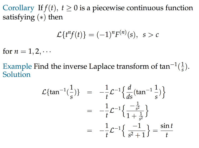
The Complete Overview of the Inverse Laplace Transform
At its core, the inverse Laplace transform is the mathematical operation that retrieves a time-domain function from its Laplace-transformed counterpart. Given a function F(s)—the Laplace transform of a signal f(t)—the inverse transform recovers f(t) via the integral:\[ f(t) = \frac{1}{2\pi i} \int_{\gamma - i\infty}^{\gamma + i\infty} e^{st} F(s) \, ds \]
This contour integral, known as the Bromwich integral, is the theoretical foundation, but practical computations often rely on residue calculus or table lookup methods. The transform’s utility stems from its ability to convert differential equations into algebraic expressions, where solutions in the s-domain can later be inverted back to the time domain.
The inverse Laplace transform is not a standalone operation but a critical link in a chain of analytical techniques. It bridges the gap between abstract algebraic manipulations and concrete time-dependent behaviors, making it indispensable in fields where system dynamics are paramount. Whether analyzing the response of a damped harmonic oscillator or designing a feedback controller, the ability to invert F(s) back to f(t) is what transforms theoretical models into actionable engineering solutions.
Historical Background and Evolution
The Laplace transform’s origins trace back to the 18th century, with contributions from mathematicians like Pierre-Simon Laplace and Joseph Fourier. However, the inverse transform’s systematic development emerged in the early 20th century as engineers sought to tackle increasingly complex differential equations. The Bromwich integral, formulated in 1918, provided the rigorous mathematical framework for inversion, but its practical application remained limited until the advent of computational tools.The mid-20th century marked a turning point, as control theorists like Rudolf Kalman and engineers at Bell Labs adopted the inverse Laplace transform to analyze stability and transient responses. The rise of digital computing further democratized its use, enabling numerical inversion techniques like the Fast Fourier Transform (FFT)-based methods. Today, the inverse Laplace transform is not just a theoretical construct but a computational workhorse, embedded in software like MATLAB, Mathematica, and SciPy.
Core Mechanisms: How It Works
The inverse Laplace transform operates under two primary mechanisms: analytical inversion and numerical approximation. Analytical methods, such as partial fraction decomposition, leverage the linearity of the transform to break down F(s) into simpler components whose inverses are known from standard tables. For example, a rational function F(s) = (s + a)/(s² + b²) can be decomposed into terms whose inverses correspond to exponential and sinusoidal functions in the time domain.Table of Contents
- The Complete Overview of the Inverse Laplace Transform
- Historical Background and Evolution
- Core Mechanisms: How It Works
- Key Benefits and Crucial Impact
- Major Advantages
- Comparative Analysis
- Future Trends and Innovations
- Conclusion
- Comprehensive FAQs
- Q: What is the difference between the Laplace transform and its inverse?
- Q: Can the inverse Laplace transform be applied to non-rational functions?
- Q: How does partial fraction decomposition aid in inversion?
- Q: What are common pitfalls when computing the inverse Laplace transform?
- Q: How is the inverse Laplace transform used in control theory?
- Q: Are there software tools that automate the inverse Laplace transform?
- Q: Can the inverse Laplace transform be extended to distributions or generalized functions?
Numerical methods, on the other hand, approximate the Bromwich integral using techniques like the Gaver-Stehfest algorithm or Euler’s method. These approaches are essential when dealing with functions that resist analytical decomposition, such as those arising from nonlinear differential equations. The choice between analytical and numerical inversion depends on the problem’s complexity, with the former offering exact solutions and the latter providing flexibility for intractable cases.
Key Benefits and Crucial Impact
The inverse Laplace transform is the linchpin of system analysis, offering unparalleled advantages in modeling and solving real-world problems. Its ability to convert differential equations into algebraic forms simplifies the study of dynamic systems, from mechanical vibrations to biological signal processing. Without it, engineers would be forced to grapple with complex time-domain solutions, delaying innovation in fields where rapid prototyping is critical.The transform’s impact extends beyond engineering into pure mathematics, where it serves as a tool for proving theorems in functional analysis and complex variables. Its role in control theory cannot be overstated: modern PID controllers, adaptive filters, and state-space representations all rely on the inverse Laplace transform to ensure stability and performance. The quote below captures its essence:
"The Laplace transform is a mathematical microscope, allowing us to peer into the hidden dynamics of systems. Its inverse is the lens that brings those dynamics back into focus, revealing the true nature of signals obscured by algebraic complexity." — John G. Truxal, Automatic Feedback Control System Synthesis
Major Advantages
- Simplification of Differential Equations: Converts PDEs and ODEs into algebraic equations, reducing complexity in system modeling.
- Stability Analysis: Enables the use of the s-plane (Root Locus, Nyquist plots) to assess system stability without solving time-domain equations.
- Signal Processing: Critical in designing filters, solving convolution integrals, and analyzing transient responses in circuits.
- Control Theory: Forms the basis for transfer function analysis, where the inverse transform recovers system outputs from input specifications.
- Numerical Flexibility: Modern algorithms allow inversion of functions that defy analytical methods, expanding its applicability to nonlinear systems.

Comparative Analysis
While the inverse Laplace transform is powerful, it is not the only tool for analyzing dynamic systems. Below is a comparison with alternative methods:| Inverse Laplace Transform | Alternative Methods |
|---|---|
| Best for linear time-invariant (LTI) systems with known F(s). | Numerical integration (e.g., Runge-Kutta) for nonlinear systems. |
| Requires knowledge of complex analysis for exact solutions. | Fourier transform for periodic signals (but lacks transient analysis). |
| Exact solutions possible for rational F(s). | State-space methods for multi-input/multi-output (MIMO) systems. |
| Limited to causal systems (t ≥ 0). | Wavelet transforms for non-stationary signal analysis. |
Future Trends and Innovations
The future of the inverse Laplace transform lies in its integration with machine learning and hybrid computational methods. As deep learning models are trained to approximate inverse transforms, the need for manual residue calculations may diminish, particularly in real-time applications like autonomous systems. Additionally, advancements in symbolic computation (e.g., Wolfram Alpha’s symbolic inversion) are pushing the boundaries of what can be solved analytically.Another frontier is the application of the inverse Laplace transform in quantum mechanics and statistical physics, where it aids in solving master equations and analyzing stochastic processes. The transform’s adaptability ensures its relevance in emerging fields, from bioengineering to renewable energy systems, where dynamic modeling remains a cornerstone of innovation.

Conclusion
The inverse Laplace transform is more than a mathematical curiosity; it is a fundamental tool that underpins modern engineering and scientific discovery. Its ability to decode complex systems into manageable algebraic forms has revolutionized how we analyze and design dynamic processes. As computational methods evolve, its role will only grow, bridging the gap between abstract theory and practical application.For engineers, physicists, and mathematicians, mastering the inverse Laplace transform is not just about solving equations—it is about unlocking the hidden dynamics of the world around us. Whether through analytical rigor or numerical innovation, its principles will continue to shape the future of system analysis.
Comprehensive FAQs
Q: What is the difference between the Laplace transform and its inverse?
The Laplace transform converts a time-domain function f(t) into a complex frequency-domain function F(s), while the inverse Laplace transform reverses this process, retrieving f(t) from F(s). The forward transform is defined as an integral over time; the inverse is a contour integral over the complex plane.
Q: Can the inverse Laplace transform be applied to non-rational functions?
Analytical inversion is typically limited to rational functions (ratios of polynomials), but numerical methods like the Gaver-Stehfest algorithm can approximate inverses for more complex F(s), including those with essential singularities or branch cuts.
Q: How does partial fraction decomposition aid in inversion?
Partial fraction decomposition breaks down F(s) into simpler terms (e.g., 1/(s + a), 1/(s² + b²)) whose inverses are known from standard tables. This reduces the problem to a sum of elementary transforms, making inversion straightforward.
Q: What are common pitfalls when computing the inverse Laplace transform?
Pitfalls include misidentifying poles (leading to incorrect residues), overlooking convergence conditions (e.g., Re(s) > σ), and assuming all functions have analytical inverses (some require numerical techniques). Improper handling of repeated roots or branch cuts can also yield incorrect results.
Q: How is the inverse Laplace transform used in control theory?
In control theory, the inverse transform recovers the time-domain response of a system from its transfer function G(s) = Y(s)/U(s). This is critical for designing controllers, analyzing stability (via root locus), and predicting system behavior under different inputs.
Q: Are there software tools that automate the inverse Laplace transform?
Yes, tools like MATLAB’s ilaplace, Mathematica’s InverseLaplaceTransform, and SciPy’s scipy.special module provide automated inversion. These use a combination of symbolic computation and numerical algorithms to handle a wide range of F(s).
Q: Can the inverse Laplace transform be extended to distributions or generalized functions?
Yes, through the theory of distributions (e.g., Dirac delta functions), the inverse Laplace transform can handle impulses and other singularities. This extension is vital in signal processing, where idealized signals (like step functions) are common.
Leave a Comment
Comments are moderated before appearing. The data you submit is processed according to the Privacy Policy of Gouv.