Understanding what is the box plot: The definitive guide to data visualization
Data analysis isn’t just about numbers—it’s about revealing patterns hidden in distributions. When researchers or analysts encounter datasets with hundreds or thousands of observations, they need tools that distill complexity into immediate insights. That’s where the box plot comes in: a deceptively simple yet profoundly effective visualization that transforms raw data into a snapshot of variability, outliers, and central tendency. Unlike histograms that show frequency or scatter plots that map individual points, what is the box plot asks a different question: How are the values spread, and where do the most meaningful thresholds lie? This isn’t just another statistical tool—it’s a decision-making compass for fields ranging from finance to healthcare.
The power of the box plot lies in its ability to communicate five critical pieces of information at once: the median, quartiles, interquartile range (IQR), potential outliers, and overall data skewness. A single glance can reveal whether a dataset is symmetric or skewed, whether most values cluster tightly or sprawl widely, and whether extreme values warrant further investigation. Yet despite its ubiquity in academic research, business analytics, and scientific reporting, many professionals still underutilize it—or misunderstand its nuances. The misconception that what is the box plot is merely a "fancy bar chart" persists, obscuring its role as a cornerstone of exploratory data analysis.
What makes the box plot uniquely valuable is its balance of simplicity and depth. While a bar chart might show average performance across categories, a box plot exposes the distribution behind those averages—revealing hidden risks, inconsistencies, or opportunities. For example, in quality control, a box plot might expose that while a manufacturing process meets average specifications, 25% of batches consistently fall outside acceptable tolerance levels. In medicine, it could highlight that while patient recovery times cluster around a median, a small but critical subgroup experiences prolonged delays. The tool’s versatility extends beyond descriptive statistics; it’s equally indispensable for hypothesis testing, outlier detection, and even comparative analysis across multiple datasets.

The Complete Overview of What Is the Box Plot
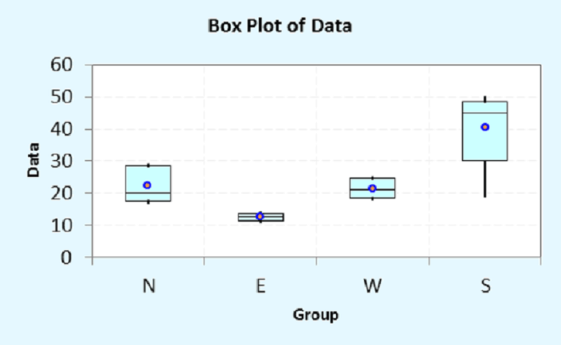
At its core, what is the box plot refers to a standardized method for visualizing the five-number summary of a dataset: the minimum, first quartile (Q1), median (Q2), third quartile (Q3), and maximum. These five values form the "box-and-whisker" structure that gives the plot its name. The "box" itself spans from Q1 to Q3, capturing the middle 50% of the data—the interquartile range (IQR)—while the median is marked by a line inside the box. The "whiskers" extend to the smallest and largest values within 1.5 times the IQR from the quartiles, with any data points beyond this range plotted individually as potential outliers. This design isn’t arbitrary; it’s rooted in robust statistical principles that minimize the influence of extreme values while maximizing clarity.The genius of the box plot lies in its ability to convey distribution shape, spread, and central tendency in a single, compact format. Unlike a histogram, which requires binning decisions that can distort perception, or a scatter plot, which can overwhelm with individual data points, the box plot abstracts the essential characteristics of a distribution. For instance, a symmetric box plot with equal whisker lengths suggests a normal distribution, while a skewed box plot with one whisker significantly longer than the other indicates asymmetry. Even the position of the median within the box reveals skewness: if the median is closer to Q1, the data is left-skewed; if closer to Q3, right-skewed. This visual intuition is why what is the box plot remains a staple in fields where quick, actionable insights are paramount.
Historical Background and Evolution
The origins of what is the box plot can be traced back to the late 19th century, when statisticians sought ways to visualize data distributions more intuitively than raw tables or frequency polygons. John Tukey, the pioneering mathematician and computer scientist, formalized the modern box plot in his 1977 book Exploratory Data Analysis. Tukey’s innovation was to combine the five-number summary with a graphical representation that emphasized the IQR, making it easier to identify outliers and assess variability. Before Tukey, visualizations like stem-and-leaf plots or dot plots dominated, but they lacked the box plot’s ability to highlight central tendencies and dispersion simultaneously.Tukey’s work wasn’t just theoretical—it was practical. He designed the box plot as a tool for exploratory analysis, where the goal is to discover patterns rather than confirm hypotheses. This aligned with the growing field of data science, where researchers needed methods to handle messy, real-world datasets. Over time, the box plot evolved beyond its exploratory roots. Software like R, Python (via libraries such as Matplotlib and Seaborn), and statistical packages in Excel integrated it as a standard feature, democratizing access to this powerful visualization. Today, what is the box plot is as likely to appear in a corporate dashboard as it is in a peer-reviewed journal, reflecting its adaptability across disciplines.
Core Mechanisms: How It Works
The mechanics of what is the box plot are straightforward but built on precise statistical definitions. The five-number summary forms the backbone: the minimum and maximum values (excluding outliers) define the whiskers, while Q1, Q2 (median), and Q3 delineate the box. Q1 is the 25th percentile—the value below which 25% of the data falls—while Q3 is the 75th percentile. The IQR, calculated as Q3 minus Q1, measures the spread of the central 50% of the data. Whiskers extend to the smallest and largest values within 1.5 × IQR from the quartiles, a threshold set to balance sensitivity to outliers with robustness to noise.Table of Contents
- The Complete Overview of What Is the Box Plot
- Historical Background and Evolution
- Core Mechanisms: How It Works
- Key Benefits and Crucial Impact
- Major Advantages
- Comparative Analysis
- Future Trends and Innovations
- Conclusion
- Comprehensive FAQs
- Q: How do I create a box plot in Excel?
- Q: Can a box plot show negative values?
- Q: What’s the difference between a box plot and a violin plot?
- Q: Why are outliers important in box plots?
- Q: How do I interpret a box plot with a very long whisker?
- Q: Are box plots useful for time-series data?
- Q: Can I use a box plot for categorical data?
- Q: What’s the relationship between box plots and the IQR?
- Q: How do I handle multiple box plots in one graph?
- Q: Are there alternatives to the 1.5 × IQR rule for outliers?
Outliers are any data points beyond the whiskers, typically flagged for further investigation. The choice of 1.5 × IQR as the outlier threshold is a convention, not a rule; some fields use stricter (e.g., 3 × IQR) or looser criteria depending on the context. The median’s position within the box is equally telling: in a symmetric distribution, it divides the box evenly, but skewness shifts it toward the shorter whisker. This interplay of elements—box, whiskers, median, and outliers—creates a visualization that’s both mathematically rigorous and intuitively graspable, answering what is the box plot in both technical and practical terms.
Key Benefits and Crucial Impact
The box plot’s enduring relevance stems from its ability to distill complex datasets into actionable insights with minimal cognitive load. In an era where data volumes are exploding, tools that reduce information overload are invaluable. A single box plot can replace pages of summary statistics, making it easier for stakeholders—from executives to clinicians—to spot trends, anomalies, or inconsistencies at a glance. For example, in supply chain management, box plots of delivery times across regions can reveal which logistics hubs are underperforming, while in clinical trials, they might expose unexpected variability in patient responses to a treatment. The tool’s strength lies in its dual role: it’s both a diagnostic tool for identifying issues and a communication device for presenting findings clearly.Beyond its practical utility, what is the box plot also fosters statistical literacy. By making distributions tangible, it helps analysts and decision-makers move beyond superficial metrics like means or medians to understand the underlying variability. This is particularly critical in fields where assumptions of normality (e.g., in parametric tests) may not hold. For instance, a box plot might reveal that a dataset is heavily skewed, prompting the use of non-parametric tests or transformations. The tool’s versatility extends to comparative analysis, where side-by-side box plots can reveal differences between groups—such as before-and-after scenarios or treatment vs. control conditions—with greater clarity than traditional bar charts.
"The box plot is not just a visualization; it’s a conversation starter between data and decision-makers. It asks questions the mean can’t: Where is the bulk of the data? Are there hidden risks? How consistent is the performance?" — John Tukey, Statistician and Data Analysis Pioneer
Major Advantages
- Compact Representation: Condenses an entire dataset’s distribution into a single, interpretable graphic, reducing information overload compared to raw data or histograms.
- Outlier Detection: Explicitly identifies extreme values beyond the whiskers, flagging potential data errors or rare events that merit investigation.
- Comparative Analysis: Enables side-by-side comparisons of multiple datasets (e.g., pre- and post-intervention) to highlight shifts in central tendency or variability.
- Robustness to Sample Size: Performs well with both small and large datasets, unlike histograms that require binning decisions or scatter plots that become cluttered.
- Statistical Rigor: Based on percentiles and IQR, it provides a non-parametric alternative to assumptions like normality, making it suitable for skewed or bimodal distributions.

Comparative Analysis
| Feature | Box Plot | Histogram |
|---|---|---|
| Primary Purpose | Visualize distribution shape, spread, and outliers. | Show frequency of values within bins. |
| Key Metrics Displayed | Median, quartiles, IQR, outliers. | Frequency counts per bin. |
| Best For | Comparing groups, detecting outliers, non-normal data. | Understanding data frequency, identifying modality. |
| Limitations | Less precise for exact value frequencies; whisker length depends on IQR. | Sensitive to bin width choices; can obscure outliers. |
Future Trends and Innovations
As data science evolves, so too will the applications of what is the box plot. One emerging trend is the integration of interactive box plots in dashboards, where users can hover over elements to see exact values or drill down into subsets of data. Tools like Plotly and Tableau are already enabling dynamic box plots that update in real time, allowing analysts to explore trends as new data streams in. Another innovation is the fusion of box plots with other visualizations, such as combining them with violin plots to show both distribution and density, or pairing them with scatter plots to reveal relationships between variables.The rise of big data and machine learning may also redefine the box plot’s role. While traditional box plots excel with univariate data, future iterations could incorporate multivariate distributions or even high-dimensional embeddings, making them more relevant in fields like genomics or NLP. Additionally, as AI-driven analytics tools become more accessible, the box plot could serve as a "sanity check" visualization—helping users validate the outputs of black-box models by revealing unexpected patterns or outliers. The core principle of what is the box plot—simplifying complexity—will remain, but its implementation will grow more sophisticated.
Conclusion
The box plot is more than a statistical artifact; it’s a testament to the power of thoughtful design in data visualization. By focusing on the five-number summary and outliers, it cuts through the noise to reveal what matters most: the distribution’s shape, spread, and potential anomalies. Whether you’re analyzing customer satisfaction scores, manufacturing tolerances, or clinical trial results, the box plot provides a lens to see beyond averages and medians to the full spectrum of variability. Its simplicity is its strength—anyone can interpret it, yet its depth allows experts to extract nuanced insights.As data continues to grow in volume and complexity, tools like the box plot will only become more essential. They bridge the gap between raw data and actionable decisions, making them indispensable in research, business, and policy-making. Understanding what is the box plot isn’t just about mastering a visualization technique; it’s about adopting a mindset that values distribution over averages, variability over uniformity, and clarity over clutter.
Comprehensive FAQs
Q: How do I create a box plot in Excel?
A: In Excel, select your data range, go to the Insert tab, and choose Insert Statistic Chart > Box and Whisker. Alternatively, use the Data Analysis Toolpak (enable via File > Options > Add-ins) to generate a box plot from summary statistics. For dynamic updates, consider using PivotCharts with a box plot template.
Q: Can a box plot show negative values?
A: Yes, box plots can display negative values as long as the data includes them. The whiskers, box, and median will adjust accordingly, though the interpretation remains the same—negative values are simply part of the distribution’s range.
Q: What’s the difference between a box plot and a violin plot?
A: While both visualize distributions, a violin plot adds a kernel density estimate to show the probability density of the data at different values, creating a symmetric, violin-like shape. A box plot, by contrast, focuses on quartiles and outliers without density information.
Q: Why are outliers important in box plots?
A: Outliers in box plots indicate data points that deviate significantly from the rest of the distribution. They can signal errors (e.g., data entry mistakes), rare events, or critical insights (e.g., a patient with an adverse reaction in clinical trials). Ignoring them risks misrepresenting the dataset’s true variability.
Q: How do I interpret a box plot with a very long whisker?
A: A long whisker suggests high variability in the data outside the IQR. If one whisker is significantly longer than the other, it indicates skewness—either left-skewed (longer lower whisker) or right-skewed (longer upper whisker). This can imply uneven distribution or the presence of extreme values in one direction.
Q: Are box plots useful for time-series data?
A: Box plots are less common for time-series analysis than line charts or control charts, but they can be useful for visualizing distributions at specific time points (e.g., monthly sales variability). For trends over time, consider combining box plots with a timeline or using rolling box plots to track changes in distribution shape.
Q: Can I use a box plot for categorical data?
A: Yes, but only if the categories represent distinct groups (e.g., "Treatment A" vs. "Treatment B"). Each category gets its own box plot, allowing side-by-side comparisons of distributions. Avoid using box plots for ordinal data unless the categories have meaningful numerical differences.
Q: What’s the relationship between box plots and the IQR?
A: The IQR (Q3 – Q1) is the foundation of the box plot. It defines the height of the box and the length of the whiskers (1.5 × IQR). The IQR is also used to calculate the outlier threshold, making it a critical measure of statistical dispersion in the visualization.
Q: How do I handle multiple box plots in one graph?
A: To compare multiple datasets, create a side-by-side box plot, ensuring each dataset has its own box and whiskers. Use consistent colors or labels to avoid confusion. Tools like R’s ggplot2 or Python’s Seaborn make this easy with faceting or grouping options.
Q: Are there alternatives to the 1.5 × IQR rule for outliers?
A: Yes, some fields use stricter (e.g., 3 × IQR) or looser thresholds (e.g., 1 × IQR) depending on the data’s sensitivity to outliers. Domain-specific rules may also apply, such as using domain knowledge to define "acceptable" ranges in manufacturing or finance.
Leave a Comment
Comments are moderated before appearing. The data you submit is processed according to the Privacy Policy of Gouv.