The Hidden Symmetry: Decoding the x^3 Graph’s Role in Math and Science
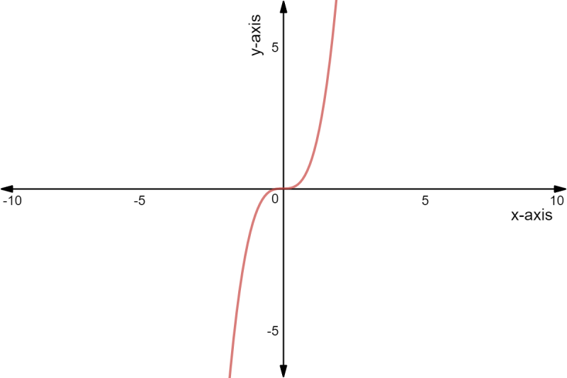
The x3 graph is more than a simple curve—it’s a fundamental building block of mathematics, a silent architect of natural phenomena, and a tool that bridges abstract theory with tangible reality. Its S-shaped trajectory, emerging from negative infinity, flattening at the origin, and soaring upward, defies the linear predictability of its quadratic cousin. This asymmetry isn’t arbitrary; it encodes the nonlinear dynamics that govern everything from the trajectory of a falling object to the behavior of neural networks in artificial intelligence. Engineers rely on it to model stress in materials, economists use it to project growth patterns, and physicists decode its implications in quantum mechanics. Yet for all its utility, the x3 graph remains an underappreciated marvel—a visual representation of how cubic relationships reshape our understanding of the universe.
What makes the x3 graph particularly fascinating is its duality: it’s both a product of pure mathematical abstraction and a mirror reflecting the chaos of real-world systems. Unlike the parabolic symmetry of quadratic equations, the cubic function’s inflection point at (0,0) introduces a critical turning point, where concavity shifts from concave-down to concave-up. This property alone explains why cubic equations are indispensable in fields ranging from fluid dynamics to cryptography. The graph’s ability to model both bounded and unbounded behaviors—whether describing the spread of an epidemic or the optimization of a supply chain—makes it a cornerstone of applied mathematics. But its power isn’t just functional; it’s aesthetic. The smooth, continuous flow of the curve embodies the harmony of calculus, where derivatives and integrals intertwine to reveal deeper truths.
The x3 graph’s influence extends beyond textbooks into the fabric of modern technology. In computer graphics, it smooths transitions between keyframes in animations; in robotics, it dictates the precision of motion trajectories; and in economics, it predicts the inflection points of market bubbles. Even in biology, the cubic relationship between variables like drug dosage and physiological response helps researchers design safer treatments. Yet despite its ubiquity, the graph’s origins are rooted in centuries of intellectual curiosity—a journey from ancient algebraic puzzles to the digital algorithms powering today’s innovations.

The Complete Overview of the x3 Graph
At its core, the x3 graph represents the function f(x) = x3, a cubic polynomial where each term’s exponent increases by one, culminating in the variable raised to the third power. This seemingly simple equation belies a complexity that distinguishes it from linear or quadratic functions. The graph’s defining feature is its point of inflection at the origin (0,0), where the curvature changes from concave downward (for x < 0) to concave upward (for x > 0). This transition isn’t just a mathematical quirk—it’s a physical principle. In nature, similar inflection points mark thresholds: the moment a dam’s stress shifts from compression to tension, or when a chemical reaction transitions from exothermic to endothermic. The x3 graph’s symmetry about the origin (odd function property) ensures that for every positive y, there’s a corresponding negative y, a balance that underpins many equilibrium models in science.Beyond its geometric properties, the x3 graph is a gateway to understanding higher-order polynomials. While linear and quadratic functions can be solved with straightforward formulas, cubics introduce the need for numerical methods or Cardano’s formula—a testament to their increased complexity. This complexity is what makes them indispensable in real-world scenarios where relationships aren’t neatly linear. For instance, in structural engineering, the cubic term in beam deflection equations accounts for the nonlinear stress distribution under load. Similarly, in machine learning, cubic activation functions in neural networks enable models to approximate more intricate patterns than their linear counterparts. The graph’s ability to capture both gradual and abrupt changes—its "S" shape—makes it a universal language for describing systems where small inputs can lead to disproportionate outputs, a phenomenon observed in everything from population growth to financial crashes.
Historical Background and Evolution
The study of cubic equations traces back to ancient Babylonian and Greek mathematicians, who grappled with geometric solutions to problems involving volumes and areas. However, it was the 16th-century Italian mathematicians—most notably Scipione del Ferro, Niccolò Fontana Tartaglia, and Gerolamo Cardano—who cracked the code for solving general cubic equations. Cardano’s 1545 work Ars Magna introduced the world to the cubic formula, a breakthrough that required complex numbers and laid the groundwork for modern algebra. Yet, the graphical representation of x3 as a continuous curve didn’t emerge until the 17th century, when René Descartes formalized the Cartesian plane. His innovation allowed mathematicians to visualize equations as geometric shapes, transforming abstract algebra into a tangible tool for analysis.The x3 graph’s evolution is intertwined with the development of calculus. Isaac Newton and Gottfried Wilhelm Leibniz independently discovered calculus in the late 17th century, and their work revealed the deep connection between cubic functions and their derivatives. Newton’s Method of Fluxions demonstrated how the slope of the x3 graph (its derivative, 3x2) changes at every point, while Leibniz’s notation (dy/dx) provided a systematic way to analyze these changes. By the 19th century, mathematicians like Augustin-Louis Cauchy and Bernhard Riemann expanded on these ideas, using cubic approximations to study the behavior of functions near critical points. Today, the x3 graph isn’t just a static image—it’s a dynamic model, constantly refined by computational tools that simulate its behavior in real time, from climate modeling to stock market forecasting.
Core Mechanisms: How It Works
The mechanics of the x3 graph hinge on its defining equation, f(x) = x3, which can be rewritten in its expanded form: f(x) = x·x·x. This multiplication of three identical variables introduces a nonlinear relationship where the output grows exponentially relative to the input. For example, doubling x from 2 to 4 increases f(x) from 8 to 64—a 700% jump, whereas a linear function would only double the output. The graph’s inflection point at (0,0) is where the second derivative (f''(x) = 6x) changes sign, indicating a shift from decelerating growth (for negative x) to accelerating growth (for positive x). This property is critical in optimization problems, where identifying such inflection points can mean the difference between success and failure in resource allocation.Table of Contents
- The Complete Overview of the x 3 Graph
- Historical Background and Evolution
- Core Mechanisms: How It Works
- Key Benefits and Crucial Impact
- Major Advantages
- Comparative Analysis
- Future Trends and Innovations
- Conclusion
- Comprehensive FAQs
- Q: Why does the x 3 graph have an S-shape, while quadratic graphs are parabolas?
- Q: Can the x 3 graph be used to model exponential growth?
- Q: How do engineers use the x 3 graph in structural analysis?
- Q: Is the x 3 graph always symmetric about the origin?
- Q: Why are cubic splines preferred over linear interpolation in data visualization?
- Q: How does the x 3 graph relate to the concept of "diminishing returns" in economics?
- Q: Are there any real-world systems where the x 3 graph doesn’t apply?
The graph’s symmetry is another key mechanism. Since f(-x) = -f(x), the x3 function is odd, meaning it’s mirrored across the origin. This symmetry ensures that every solution to x3 = k has exactly one real root for any real k, a guarantee absent in even-degree polynomials like quadratics. This uniqueness is why cubic equations are favored in root-finding algorithms, such as the Newton-Raphson method, which iteratively approximates solutions by leveraging the graph’s smooth, continuous nature. Additionally, the graph’s asymptotic behavior—approaching negative infinity as x → -∞ and positive infinity as x → +∞—mirrors the unbounded nature of many physical systems, from cosmic expansion to economic inflation.
Key Benefits and Crucial Impact
The x3 graph’s influence spans disciplines, offering solutions where linear or quadratic models fail. In physics, it models the relationship between force and displacement in elastic materials, where Hooke’s Law (F = kx) breaks down under large stresses. In economics, cubic functions capture the diminishing returns of investment, where initial capital yields high returns, but additional inputs produce progressively smaller gains. Even in biology, the cubic term in the Hill equation describes the saturation kinetics of enzyme-substrate reactions. These applications underscore the graph’s versatility, but its true power lies in its ability to interpolate—to smoothly connect discrete data points in a way that linear regression cannot. This interpolation is the backbone of spline functions in computer-aided design (CAD), where cubic splines ensure smooth transitions between control points in 3D modeling.The x3 graph also plays a pivotal role in error correction and signal processing. In digital communications, cubic phase correction algorithms mitigate distortions in transmitted signals, while in image processing, cubic interpolation enhances resolution without introducing artifacts. The graph’s mathematical properties—its continuity, differentiability, and invertibility—make it ideal for these tasks. As John von Neumann once noted:
"The purpose of computing is insight, not numbers." The x3 graph embodies this philosophy, transforming raw data into intuitive visualizations that reveal patterns hidden in the noise.
Major Advantages
- Nonlinear Modeling: Captures real-world relationships where inputs and outputs aren’t proportional, such as population growth or chemical reactions.
- Unique Root Guarantee: Every cubic equation has at least one real root, ensuring solutions exist for optimization problems in engineering and economics.
- Smooth Interpolation: Used in spline functions to create seamless transitions in graphics, animation, and data fitting.
- Inflection Point Analysis: Identifies critical thresholds in systems, from structural stress points to market trend reversals.
- Derivative Properties: Its first and second derivatives provide insights into rate of change and concavity, essential for calculus-based fields like physics and finance.
Comparative Analysis
| Feature | x3 Graph | Quadratic Graph (x2) |
|---|---|---|
| Shape | S-shaped (concave down → concave up) | Parabolic (always concave up or down) |
| Roots | Always one real root (three total, counting complex) | Zero, one, or two real roots |
| Symmetry | Odd function (symmetric about origin) | Even function (symmetric about y-axis) |
| Applications | Nonlinear optimization, splines, phase correction | Projectile motion, profit maximization, area calculations |
Future Trends and Innovations
As computational power grows, the x3 graph is poised to become even more integral to machine learning and quantum computing. Current neural networks rely on cubic activation functions (like ReLU variants) to introduce nonlinearity, but future architectures may exploit higher-order cubic approximations for more efficient training. In quantum algorithms, cubic interpolation could optimize qubit state transitions, reducing errors in quantum simulations. Meanwhile, biomorphic design—where engineers mimic natural cubic growth patterns—is revolutionizing materials science, leading to lighter, stronger structures inspired by the x3 graph’s inflection-driven behavior.The graph’s role in climate modeling is another frontier. Cubic equations help simulate the nonlinear feedback loops in Earth’s systems, such as ice-albedo effects or ocean current dynamics. As data resolution improves, the x3 graph’s ability to model abrupt shifts—like tipping points in ecosystems—will be critical for predicting catastrophic scenarios. Even in artificial general intelligence (AGI), the graph’s properties may underpin self-correcting algorithms that adapt to unpredictable environments, much like the cubic function’s own adaptive curvature.

Conclusion
The x3 graph is far more than a mathematical curiosity—it’s a lens through which we interpret the nonlinear world. From its historical roots in algebraic breakthroughs to its modern applications in AI and climate science, the graph’s S-shaped elegance solves problems that linear thinking cannot. Its inflection point, symmetry, and unbounded growth make it a universal tool, bridging abstract theory with practical innovation. As fields like quantum computing and biomimicry advance, the x3 graph will continue to evolve, remaining a testament to mathematics’ power to illuminate the hidden order in chaos.Understanding this graph isn’t just about plotting points; it’s about recognizing the cubic relationships that shape our reality. Whether in the trajectory of a rocket, the folding of a protein, or the optimization of a supply chain, the x3 graph quietly orchestrates the balance between stability and transformation. Its story is one of resilience—an equation that has withstood centuries of scrutiny and will undoubtedly shape the next era of discovery.
Comprehensive FAQs
Q: Why does the x3 graph have an S-shape, while quadratic graphs are parabolas?
The S-shape arises because the cubic term (x3) introduces a point of inflection where the curve’s concavity changes. Quadratic graphs (x2) lack this term, so their curvature remains consistent (always concave up or down), forming a parabola. The inflection point in cubics occurs where the second derivative (6x) changes sign, typically at x = 0 for f(x) = x3.
Q: Can the x3 graph be used to model exponential growth?
No, the x3 graph represents polynomial (power-law) growth, not exponential. Exponential growth is modeled by functions like f(x) = ax, where the variable is in the exponent. Cubic growth (x3) increases at a rate proportional to x2, whereas exponential growth accelerates much faster. However, for small x, a cubic function can approximate exponential behavior in certain contexts (e.g., Taylor series expansions).
Q: How do engineers use the x3 graph in structural analysis?
Engineers use cubic equations to model beam deflection under load, where the relationship between force and displacement isn’t linear. The Euler-Bernoulli beam theory incorporates cubic terms to account for bending moments and shear forces. The graph’s inflection point helps identify critical stress concentrations, ensuring structures like bridges or aircraft wings can withstand dynamic loads without failing.
Q: Is the x3 graph always symmetric about the origin?
Yes, the standard f(x) = x3 is symmetric about the origin because it’s an odd function (f(-x) = -f(x)). However, transformations like f(x) = x3 + k (vertical shift) or f(x) = (x - h)3 (horizontal shift) break this symmetry. The graph retains its S-shape but shifts position, which is why general cubic functions are written as f(x) = ax3 + bx2 + cx + d—where b and d can distort symmetry.
Q: Why are cubic splines preferred over linear interpolation in data visualization?
Cubic splines use piecewise cubic polynomials to create smoother, more natural transitions between data points than linear interpolation. While linear interpolation connects points with straight lines (creating jagged edges), cubic splines ensure the first and second derivatives are continuous, producing curves that mimic real-world smoothness. This is critical in graphics, animation, and scientific plotting, where abrupt changes can distort trends.
Q: How does the x3 graph relate to the concept of "diminishing returns" in economics?
In economics, diminishing returns describe a situation where each additional unit of input yields progressively smaller increases in output. A cubic function like f(x) = x3 can model this if the input is scaled appropriately (e.g., f(x) = 100x - x3), where the cubic term eventually dominates, causing growth to slow. This mirrors real-world scenarios, such as fertilizer application in agriculture, where beyond a certain point, extra inputs produce marginal gains.
Q: Are there any real-world systems where the x3 graph doesn’t apply?
Yes, the x3 graph is unsuitable for systems with exponential decay/growth (e.g., radioactive decay), logarithmic relationships (e.g., sound intensity in decibels), or piecewise constant behaviors (e.g., digital signals). It also fails to model chaotic systems (like weather patterns) where small changes lead to unpredictable outcomes, as cubics are deterministic and smooth. However, in many cases, cubic approximations serve as useful local models within broader frameworks.
Leave a Comment
Comments are moderated before appearing. The data you submit is processed according to the Privacy Policy of Gouv.