Transforming Data Visualization: How to Make Color Legend Scale in COMSOL Logarithmic
The moment you open COMSOL and confront a dataset spanning orders of magnitude—whether it’s temperature gradients in a semiconductor, stress distributions in a composite material, or concentration fields in a biochemical reactor—you realize standard linear color legends fail. They compress critical details into indistinguishable bands, drowning the nuances that define your simulation’s integrity. That’s when you need to make color legend scale COMSOL logarithmic, a technique that transforms raw data into a visually intelligible spectrum where exponential variations become discernible patterns.
Logarithmic scaling isn’t just a cosmetic adjustment; it’s a methodological pivot. In fields like fluid dynamics or electromagnetic modeling, where phenomena like turbulence or field intensity follow power laws, a linear legend distorts reality. A logarithmic approach preserves proportional relationships, revealing hidden gradients that linear scales flatten into monotony. Yet, mastering this feature in COMSOL requires more than toggling a checkbox—it demands an understanding of how logarithmic transformations interact with your solver’s output, your post-processing workflow, and the very physics you’re modeling.
The challenge lies in execution. COMSOL’s interface doesn’t always advertise its logarithmic scaling capabilities upfront, and misconfigurations can lead to artifacts—ghost contours where none should exist, or misleading interpretations of your results. This guide demystifies the process, from selecting the right color map to validating your logarithmic legend against raw data. Whether you’re debugging a thermal simulation or optimizing a plasma discharge model, the ability to customize COMSOL’s color legend scale logarithmically is a skill that separates clear insights from chaotic noise.

The Complete Overview of Logarithmic Color Scaling in COMSOL
COMSOL Multiphysics provides a suite of tools to visualize simulation results, but its default linear color legends often obscure the full spectrum of data, especially when dealing with variables that span several orders of magnitude. To address this, users frequently turn to logarithmic scaling—a technique that compresses large ranges into a manageable visual format. The process of making a color legend scale logarithmic in COMSOL involves accessing hidden settings within the post-processing module, where the software allows for non-linear transformations of the color axis. This is particularly useful in scenarios involving exponential decay, multiplicative effects, or phenomena where relative changes are more critical than absolute values.
The core idea behind logarithmic scaling is to map data onto a logarithmic axis, which effectively stretches out small values while compressing large ones. This approach ensures that variations across the entire range remain visually distinguishable, rather than being clustered into a single color band. For instance, in a simulation of heat transfer through a composite material, temperature differences near the boundaries might be negligible in a linear scale but critical in a logarithmic one. By applying a logarithmic color legend scale in COMSOL, engineers can identify subtle thermal gradients that would otherwise be lost in a uniform color wash.
Historical Background and Evolution
The concept of logarithmic scaling traces back to early scientific visualization, where mathematicians and physicists sought ways to represent data that spanned multiple magnitudes. In the 19th century, log-log plots became standard in fields like astronomy and acoustics, allowing researchers to compare phenomena across vast scales. COMSOL, as a modern simulation tool, inherits this tradition but adapts it to computational modeling. Early versions of COMSOL relied on linear legends by default, reflecting the dominance of linear algebra in numerical methods. However, as simulations grew more complex—incorporating non-linear partial differential equations (PDEs)—the need for logarithmic scaling became apparent.
Table of Contents
- The Complete Overview of Logarithmic Color Scaling in COMSOL
- Historical Background and Evolution
- Core Mechanisms: How It Works
- Key Benefits and Crucial Impact
- Major Advantages
- Comparative Analysis
- Future Trends and Innovations
- Conclusion
- Comprehensive FAQs
- Q: Can I apply a logarithmic color legend to any variable in COMSOL?
- Q: How do I choose the right color map for logarithmic scaling?
- Q: Will logarithmic scaling affect the accuracy of my simulation results?
- Q: Can I automate the logarithmic color legend range in COMSOL?
- Q: What are common mistakes when using logarithmic color legends?
Today, COMSOL’s logarithmic color scaling is an evolution of these historical techniques, integrated into a user-friendly interface that abstracts the underlying mathematics. Users can now apply logarithmic transformations with minimal coding, thanks to built-in functions and graphical user interfaces (GUIs) that simplify the process. This democratization of advanced visualization techniques has empowered engineers, researchers, and students to interpret data more accurately, reducing the risk of misinterpretation due to poorly chosen color scales.
Core Mechanisms: How It Works
At its core, logarithmic scaling in COMSOL operates by transforming the data range into a logarithmic domain before mapping it to the color spectrum. When you select a logarithmic color legend, COMSOL internally applies the natural logarithm (or base-10 logarithm, depending on configuration) to the data values. This transformation ensures that equal ratios of data correspond to equal distances on the color bar. For example, a value of 10 and 100 would be equidistant from 1 on a logarithmic scale, whereas they would be 90 units apart on a linear scale.
The implementation involves two key steps: selecting the logarithmic scale option in the color legend settings and choosing an appropriate color map. COMSOL supports several color maps (e.g., "Jet," "Hot," "Parula"), but some are better suited for logarithmic scaling than others. For instance, the "Viridis" color map, which avoids abrupt color transitions, is often preferred for logarithmic visualizations. Additionally, users must specify the range of the logarithmic scale, which can be set manually or automatically based on the data’s minimum and maximum values. This flexibility ensures that the visualization accurately reflects the underlying physics, whether the data spans decades or just a few orders of magnitude.
Key Benefits and Crucial Impact
The decision to adjust COMSOL’s color legend scale to logarithmic is rarely arbitrary; it’s a deliberate choice to enhance clarity, precision, and interpretability. In fields like computational fluid dynamics (CFD) or electromagnetic simulations, where variables like velocity or electric field intensity can vary exponentially, a logarithmic scale reveals patterns that linear scales obscure. For example, in a plasma simulation, electron density might span from 10^10 to 10^18 particles per cubic meter. A linear legend would compress this range into a few indistinct colors, while a logarithmic legend preserves the full dynamic range, allowing engineers to identify critical thresholds or anomalies.
Beyond technical accuracy, logarithmic scaling also improves collaboration and communication. When presenting simulation results to stakeholders—whether they are engineers, managers, or regulators—a well-chosen color legend ensures that the data’s nuances are not lost in translation. Misleading visualizations can lead to costly errors, such as overlooking stress concentrations in a structural analysis or misinterpreting temperature distributions in a thermal management system. By leveraging a logarithmic color legend in COMSOL, users mitigate these risks, ensuring that their insights are both scientifically rigorous and practically actionable.
"Logarithmic scaling is not just a tool; it’s a language. It allows us to speak the language of exponential processes—the language of nature itself." — Dr. Elena Vasquez, Computational Physics Researcher, MIT
Major Advantages
- Preservation of Dynamic Range: Logarithmic scaling ensures that data spanning multiple orders of magnitude is represented without compression, making subtle variations visible.
- Enhanced Pattern Recognition: Exponential trends, such as those in turbulence or decay processes, become discernible, aiding in the identification of critical phenomena.
- Reduced Visual Distortion: Avoids the "crowding" effect seen in linear legends, where most data is clustered in one color band, leaving other regions underrepresented.
- Improved Data Validation: Facilitates cross-checking simulation results against theoretical models or experimental data, where logarithmic relationships are common.
- Flexibility in Interpretation: Allows users to toggle between linear and logarithmic views, enabling a more comprehensive analysis of the same dataset.
Comparative Analysis
| Feature | Linear Color Legend | Logarithmic Color Legend |
|---|---|---|
| Data Range Handling | Compresses large ranges into few colors; small variations may be indistinguishable. | Expands dynamic range; preserves proportional relationships across magnitudes. |
| Best Use Case | Variables with small dynamic ranges (e.g., temperature in a small domain). | Variables with exponential or multiplicative behavior (e.g., concentration, stress, field intensity). |
| Visual Clarity | Can obscure critical gradients; prone to "crowding" at high/low ends. | Reveals hidden gradients; avoids distortion of exponential trends. |
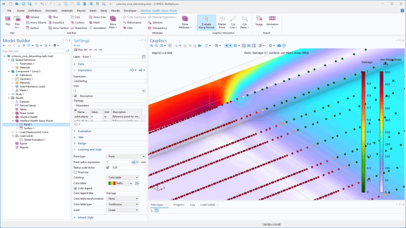
| COMSOL Implementation | Default setting; accessible via standard color axis options. | Requires manual activation in post-processing; may need custom color maps. |
Future Trends and Innovations
As COMSOL continues to evolve, so too will its visualization capabilities. Future updates may introduce more intuitive logarithmic scaling tools, such as AI-driven color map recommendations tailored to specific simulation types. Additionally, advancements in interactive visualization—like real-time logarithmic adjustments—could further streamline the workflow for engineers. The integration of machine learning to automatically detect optimal scaling parameters based on data characteristics is another promising direction, reducing the need for manual intervention.
Beyond COMSOL, the broader field of scientific visualization is moving toward more adaptive and context-aware tools. For instance, adaptive logarithmic scaling—where the scale adjusts dynamically based on user interaction or data updates—could become standard. Such innovations would not only enhance the accuracy of simulations but also democratize access to advanced visualization techniques, allowing more researchers to leverage logarithmic scaling without deep technical expertise.
Conclusion
Mastering the art of making a color legend scale logarithmic in COMSOL is more than a technical skill; it’s a gateway to deeper insights in computational modeling. Whether you’re analyzing fluid flow, thermal gradients, or electromagnetic fields, logarithmic scaling transforms raw data into a clear, actionable narrative. The key lies in understanding when and how to apply it—recognizing that not every dataset benefits from a logarithmic approach, but when it does, the difference between obscurity and clarity can be profound.
As simulations grow in complexity, the tools to interpret them must keep pace. COMSOL’s logarithmic color scaling is a testament to this evolution, bridging the gap between raw computational output and human understanding. By embracing these techniques, engineers and researchers can push the boundaries of what’s visible—and what’s achievable—in their simulations.
Comprehensive FAQs
Q: Can I apply a logarithmic color legend to any variable in COMSOL?
A: While COMSOL supports logarithmic scaling for most numeric variables, it’s not universally applicable. For example, logarithmic scaling is unsuitable for variables with zero or negative values, as the logarithm is undefined in these cases. Additionally, some physics interfaces may impose constraints on color scaling options. Always check the variable’s range and the solver’s output before applying logarithmic scaling.
Q: How do I choose the right color map for logarithmic scaling?
A: The ideal color map for logarithmic scaling should avoid abrupt transitions and provide good perceptual uniformity. "Viridis" is often recommended due to its smooth gradient and accessibility for color-blind users. Avoid maps like "Jet," which can introduce misleading color transitions. Experiment with different maps in COMSOL’s post-processing settings to see which best highlights your data’s nuances.
Q: Will logarithmic scaling affect the accuracy of my simulation results?
A: No, logarithmic scaling is purely a visualization technique and does not alter the underlying numerical results. It only changes how those results are displayed. However, misapplying logarithmic scaling (e.g., to inappropriate data ranges) can lead to misinterpretations. Always validate your visualization against raw data or alternative linear representations to ensure accuracy.
Q: Can I automate the logarithmic color legend range in COMSOL?
A: COMSOL allows you to set the logarithmic color legend range automatically based on the data’s minimum and maximum values. Navigate to the color axis settings in the post-processing module and select the "Auto" option for the scale range. This ensures the legend adapts dynamically to your simulation’s output, though manual adjustments may still be necessary for optimal clarity.
Q: What are common mistakes when using logarithmic color legends?
A: Common pitfalls include:
- Applying logarithmic scaling to data with zero or negative values.
- Using color maps with poor contrast, such as "Jet," which can obscure details.
- Ignoring the data’s physical context—logarithmic scaling may not be meaningful for linear phenomena.
- Not validating the visualization against raw data or alternative scales.
Leave a Comment
Comments are moderated before appearing. The data you submit is processed according to the Privacy Policy of Gouv.